The energy levels of a magnetic lattice are encoded in the boundaries between opposite spins

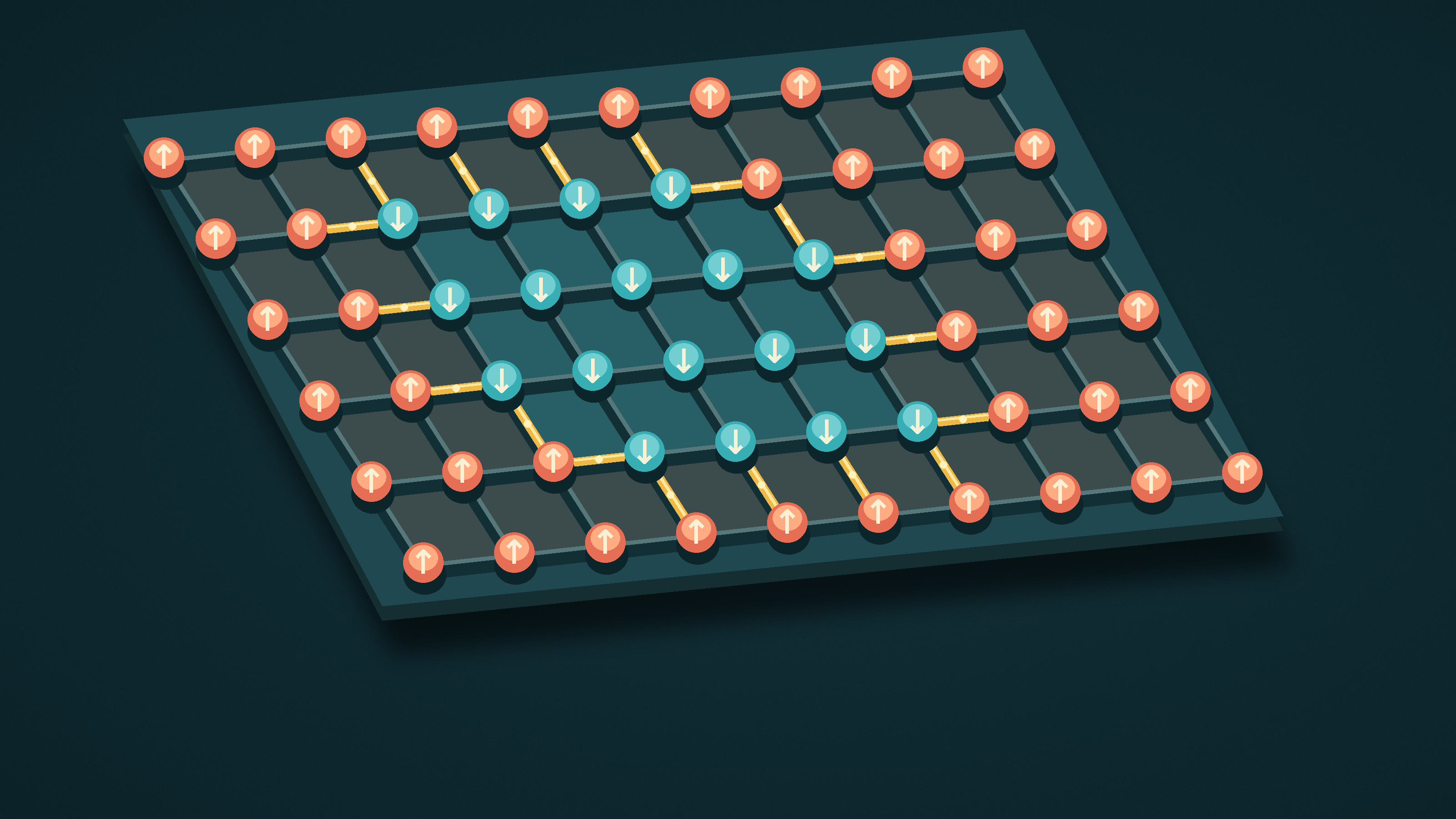
Arrange 24 spins, each of which can point only up or down, on a small lattice, and there are more than 16 million possible configurations. Yet with one particular pattern of periodic connections, these configurations fall into just 23 energy levels. Why do the vast majority of configurations end up sharing energy values, and why do some seemingly permissible energies remain unoccupied? Researchers at Gewu shift their attention from the spins to the bonds connecting them: bonds between opposite spins can both classify the energies and explain the gaps in the spectrum. A vast counting problem thus reveals a structure that can be reasoned through step by step.

Counting configurations and counting energies are different problems

Imagine a sheet of graph paper with a small arrow at every intersection. Each arrow can point only up or down, and neighboring arrows interact. If neighbors pointing in the same direction have lower energy than those pointing in opposite directions, the whole system tends to align. This is the basic way the Ising model describes ferromagnetism. The arrows here represent a simplified set of spin values; they do not mean that an electron in a real material is a little magnetic needle that can rotate freely.

The lattice discussed here is finite, and every bond between neighbors has exactly the same interaction strength. For now, there is also no external magnetic field, so neither up nor down has an inherent advantage. Each lattice site presents a binary choice: with $N$ sites, there are $2^N$ configurations in total.

But changing the directions of the arrows at the lattice sites does not necessarily change the total energy. Many different configurations share an energy, a property called degeneracy; the number of configurations with a given energy is its degeneracy. Here, an “energy level” means a distinct total energy available to these classical configurations, not a rung in an atom’s ladder of quantum transitions.

Why go to the trouble of counting these repetitions? Because thermal equilibrium does not select only the configuration with the lowest energy. At nonzero temperatures, configurations with higher energies can also occur; if many configurations share an energy, their combined probability can be substantial. Knowing only which configuration minimizes energy does not tell us how the system changes when heated. A complete classification of energies and their degeneracies separates “how likely each configuration is to occur” from “how many such configurations there are,” allowing them to be reweighted for different temperatures.

In a 2018 preprint, Rong Qiang Wei discussed the partition function of finite Ising models: the sum over all configurations, each assigned its thermal-equilibrium weight. For a 24-site example, he reported that more than 16 million terms contained only 23 distinct exponent values, leaving open the question of how to determine how many times each value occurs. Original preprint

The Gewu researchers now ask about the connectivity underlying this sum. For a class of two-dimensional square lattices that wrap around in both directions, with both side lengths even and at least four, they prove that the number of zero-field energy levels is exactly $N-1$. This result does not require listing all $2^N$ configurations one by one. The key is first to establish exactly what information about a configuration its energy retains.

Find the neighbors with opposite spins

A bond has only two possibilities: its ends point in the same direction, or in opposite directions. Let each bond between aligned spins contribute an energy of $-J$, and each bond between opposite spins contribute $+J$, where $J>0$ is the uniform interaction strength. Changing a bond from aligned to opposite spins costs an additional $2J$ in energy.

If there are $q$ bonds in total, of which $u$ connect opposite spins, the total energy is

$$\mathcal{E}=-Jq+2Ju.$$

Here, $\mathcal{E}$ is the energy of the entire configuration. The first term is the energy when all arrows point in the same direction; the second is the additional cost of bonds between opposite spins. Thus, with $q$ and $J$ fixed, knowing $u$ determines the energy, and distinct values of $u$ correspond to distinct energies.

Put all the down-spin sites in one group and the remaining, up-spin sites in another. The bonds between opposite spins are precisely the edges crossing between the two groups. In mathematics, partitioning the vertices of a connectivity graph into two groups and collecting the edges that cross between them defines a “cut”; the number of these edges is the cut size. The boundary here need not form a smooth contour in space: it simply consists of these connections between groups.

The physical question about energy levels therefore becomes two questions in graph theory: which cut sizes can this graph produce, and how many partitions produce each size? The down-spin group uniquely specifies a spin configuration, so this transformation loses no configurations.

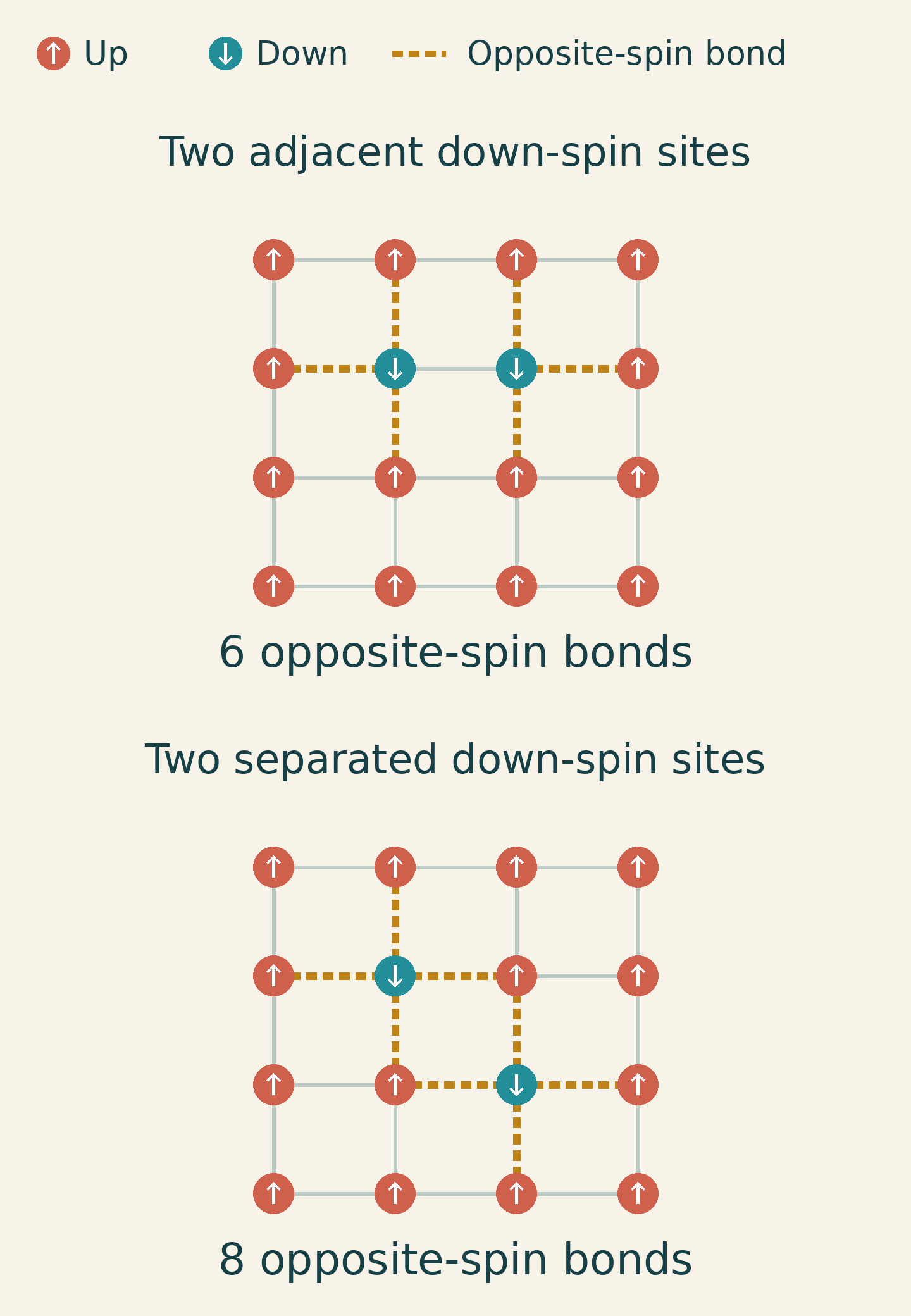
Figure 1 shows why counting down-spin sites alone is not enough. If two interior sites are separated, each has four opposite-spin bonds, for a total of eight. If they are adjacent, both ends of their shared bond point down, so it does not count toward the boundary, leaving only six in total. The number of sites has not changed, but their connectivity has changed the energy.

This also provides a practical way to count: first add up all edges incident to down-spin sites, then subtract the internal connections that were included. Each internal connection has been counted once at each end, so it must be subtracted twice. This simple observation is a starting point for deriving the structure of the entire energy spectrum.

Why some energies are always absent

Now connect the left edge of the square lattice back to the right, and the top back to the bottom. Crossing one side brings you back through the other: these are periodic boundary conditions. They specify which sites are connected; they do not require physically bending a magnetic material into a torus.

First consider a periodic square lattice with at least four sites along each side, so that every site has four bonds to neighbors. If there are $n$ down-spin sites, they have $4n$ incident edges in total. If $e$ of these connections are internal, the number of opposite-spin bonds is

$$u=4n-2e.$$

Both $n$ and $e$ are integers, so $u$ must be even. Although it may seem that energy could rise as opposite-spin bonds are added one at a time, an odd number of such bonds is in fact impossible.

Not every even number is possible, either. When all arrows point in the same direction, $u=0$; flipping just one site gives $u=4$. The connectivity of this periodic square lattice guarantees that whenever both orientations are present, at least four edges connect the two groups. This also rules out $u=2$. Intuitively, a closed row or column that passes from one group into the other must pass back again. If the boundary varies in both directions, each direction contributes at least two edges between groups. If it varies in only one direction, it must span the entire lattice, again requiring at least four connections.

When both side lengths are even, the sites can also be colored alternately in two colors, like a checkerboard, so that every bond crosses between colors. Take any spin configuration and flip only the arrows on sites of one checkerboard color. Exactly one end of every bond is then flipped. Bonds between aligned spins become bonds between opposite spins, and vice versa, turning $u$ into $q-u$.

Perform this flip twice, and the original configuration returns. Thus the operation pairs not just energy levels, but also the configurations at corresponding levels, one to one: however many configurations produce $u$ opposite-spin bonds, the same number produce $q-u$. The two ends of the zero-field energy spectrum mirror each other. Since two opposite-spin bonds are impossible, a configuration with just two fewer than the maximum possible number is impossible too.

For example, a four-by-four periodic square lattice has 16 sites and 32 bonds. The number of opposite-spin bonds can be zero or the full 32, but cannot be two or 30. Odd numbers are also excluded. Yet the crucial step remains: can every other even number occur? Knowing where levels must be absent does not tell us where configurations are guaranteed to exist.

Filling the middle of the spectrum with short segments

The Gewu researchers answer this question with a construction that can be drawn directly.

Begin with every arrow pointing up, then flip a contiguous segment of arrows in one row. Let its length be $k$, without filling the entire row. It has one opposite-spin bond at each end, and every site in the segment contributes one bond to the row above and one to the row below. The segment therefore produces $2k+2$ opposite-spin bonds. One site produces four, two sites produce six, three sites produce eight, and so on. Varying the segment length changes the bond count in even steps, and the energy changes with it.

If that is not enough, place a second segment in another row that is not adjacent to the first. With no direct connections between the segments, their boundary-edge counts add. Choosing every other row both keeps the short segments from touching and provides room for enough of them.

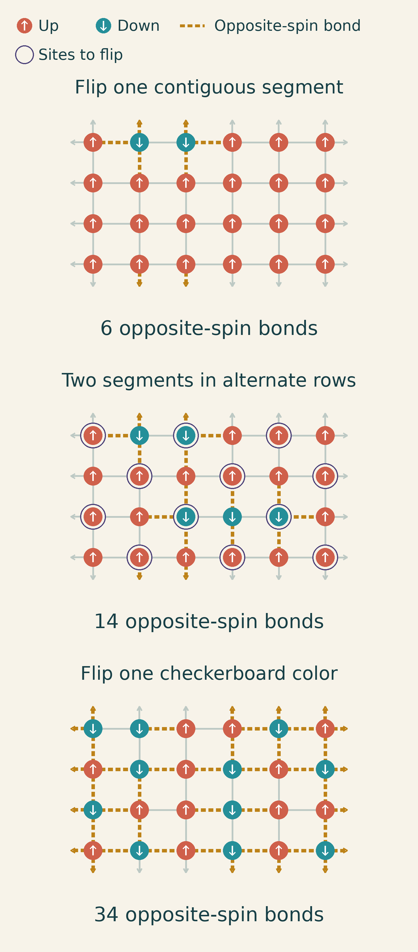
Take the six-by-four lattice in Figure 2. A single short segment can produce four, six, eight, ten, or twelve opposite-spin bonds. The total for two segments in alternate rows can take every even value from eight through 24. Together, these two ranges cover every even number from four through 24.

The same idea applies to periodic square lattices with both side lengths even and at least four. As the number of short segments increases, the achievable ranges of even numbers join up, extending all the way to half the total number of bonds. Flipping one checkerboard color then maps configurations in this half to the other half. Configurations with all bonds between aligned spins or all bonds between opposite spins supply the two endpoints.

The allowed values of $u$ are therefore all even numbers from zero through $q$, excluding only two and $q-2$. Each site in this lattice has four edges, and each edge is shared by its two ends, so the total number of bonds is $q=2N$. Counting from zero through $2N$ gives $N+1$ even numbers; removing the two gaps leaves exactly $N-1$ energy levels. The same reasoning gives 15 levels for a four-by-four lattice and 23 for a six-by-four lattice.

This is not a pattern guessed from tables for small lattices. The segment construction supplies actual configurations, the mirror flip fills in the other half, and parity and the minimum of four boundary edges establish that no other levels have been missed.

24 sites do not necessarily define the same model

We can now return to the seemingly three-dimensional 24-site example from the opening: two sites along each of two directions and six along the other, or $2\times6\times2$.

When a direction is only two sites long, periodic boundary conditions require an explicit convention: moving forward or backward from a site along that direction reaches the same neighbor. Should this pair of sites count as one bond or two? This ambiguity, which does not arise for longer lattice dimensions, directly changes the energy calculation here.

If each pair is counted as just one bond, the cross-section formed by the two directions of length two is simply four sites connected in a quadrilateral. Connecting these quadrilaterals in a periodic sequence along the direction of length six produces the same connectivity graph as a four-by-six periodic square lattice. The sites can be renumbered and rearranged while preserving every neighbor relationship.

Because energy depends only on connectivity, these two lattices, despite appearing to have different dimensionalities, have the same energy spectrum and even the same full degeneracy counts. This explains 23: it follows the $N-1$ rule for a 24-site periodic square lattice, rather than a property unique to the “three-dimensional” label.

Counting bonds twice along the periodic directions of length two changes the model. For the same 24 sites, the paper’s exact calculation gives 33 zero-field energy levels rather than 23. The original preprint does state that it uses periodic boundary conditions, but those words alone do not specify how bonds in directions of length two are counted. The present study reproduces 23 under the convention used for the comparison, and also shows why the connection rules need to accompany any quoted energy-level count for a finite lattice.

Identifying energies is easier than counting all their repetitions

Deriving the number of energy levels from connectivity does not mean that every configuration at each level has been counted. The segment construction guarantees that “at least one exists,” but does not list every possible shape and position. The study still provides no general closed-form expression for degeneracies in two or more dimensions.

To calculate them, the Gewu researchers advance through the lattice one layer at a time. They record the orientations in the current layer, together with the accumulated bond and magnetization information, then attach a new layer. Identical intermediate cases can be merged, avoiding the need to expand every configuration of the whole lattice. If the only question is whether a particular energy exists, even the configuration counts can be omitted: only “reachable” or “unreachable” need be stored.

This distinction allows the paper’s exact calculations to extend to long, narrow lattices with a thousand sites. A thousand-site ring, for example, has 501 zero-field energy levels. It has $2^{1000}$ configurations, but determining which bond counts can occur does not require visiting each configuration. Omitting the counts also avoids the problem of storing enormous degeneracies in fixed-width integers; this does not mean that large integers cannot be represented mathematically.

Lattice width remains the difficulty. The wider each layer, the more orientation combinations must be processed, and the computational cost still grows exponentially with the cross-sectional size. Thus, “reaching a thousand sites” does not mean that a thousand-site lattice of any shape is easy to handle.

The simple formula for the level count also has limits. The construction proves that even-sided periodic square lattices have no gaps in the middle, but this conclusion cannot simply be carried over to more general lattices. Of the 94 lattices reported in the paper, two still have missing levels in the middle. One 24-site lattice has 45 levels, whereas a formula assuming a completely filled middle would give 49. These gaps are related to how many internal connections small sets of sites can accommodate; they cannot be inferred from parity and the ends of the spectrum alone.

An external magnetic field brings another change. The field favors one orientation, adding $-hM$ to the total energy: $h$ is the energy scale of the uniform external field, and $M$ is the number of up-spin sites minus the number of down-spin sites. Configurations with the same number of opposite-spin bonds can then split because their $M$ values differ; different combinations of the two energy terms can also happen to coincide at particular parameter values. The paper retains a joint table of bond counts and magnetization so that results can be recalculated for different external fields. The zero-field result of 23 cannot simply be taken as the answer with a field present.

The contribution of this work is to separate “exponentially many configurations” into two problems of different difficulty. Connectivity can often establish which energy values are possible, while determining how many configurations have each value still requires finer counting. The more than 16 million configurations in the opening have not disappeared. What has changed is that we know where to look first: how many edges lie between up and down?

---

Research source: The paper on which this article is based, Exact level structure of finite uniform Ising lattices: the density of states is a cut-size spectrum, September 7, 2026; primarily Sections 5.1–5.9 and Section 8. All images are original programmatically drawn illustrations for this article; source code is available at sources/draw_figures.py.