Random quantum measurements: why are slightly fewer than a quarter incompatible?

For the same qubit, we can choose between two measurements, each answering only “yes” or “no.” Could we build a third device that measures just once, then read its record in two ways to recover the statistics that each of the first two devices would have produced? Quantum theory sometimes rules this out. Earlier numerical calculations suggested that exactly a quarter of randomly chosen measurement pairs cannot be implemented this way. Gewu researchers have now proved that the true proportion is slightly below this neat fraction. Behind the difference lies a boundary jointly determined by measurement direction, blurring, and outcome bias.

How many questions can one record answer?

A thermometer and a barometer can each produce a reading, and there is nothing surprising about entering both readings in the same table. With quantum systems, however, “combining two measurements” becomes a real question of physics.

Take electron spin as an example. Spin is an intrinsic quantum property of an electron. Measuring it along a chosen direction yields only two outcomes, usually called “up” and “down.” Measuring along the vertical direction and measuring along the horizontal direction ask different questions of the same system. A single joint measurement cannot fully replace these two ideal measurements.

“Replace” has a precise meaning here. Suppose both measurements have only two outputs, “yes” and “no.” A joint device could produce four kinds of record: “yes, yes,” “yes, no,” “no, yes,” and “no, no.” If we look only at the first answer in each record, the resulting statistics must match those of the first measurement. Looking only at the second answer must recover the statistics of the second measurement. This requirement must hold for every quantum state that could be fed into the device, rather than just one specially prepared state.

If such a joint device exists, the two measurements are called “compatible”; if no such device can be found, they are “incompatible.” This does not require performing the first measurement and then the second on the same electron. Instead, it asks whether another physical measurement exists that can supply, in one go, enough information to recover the statistics of both.

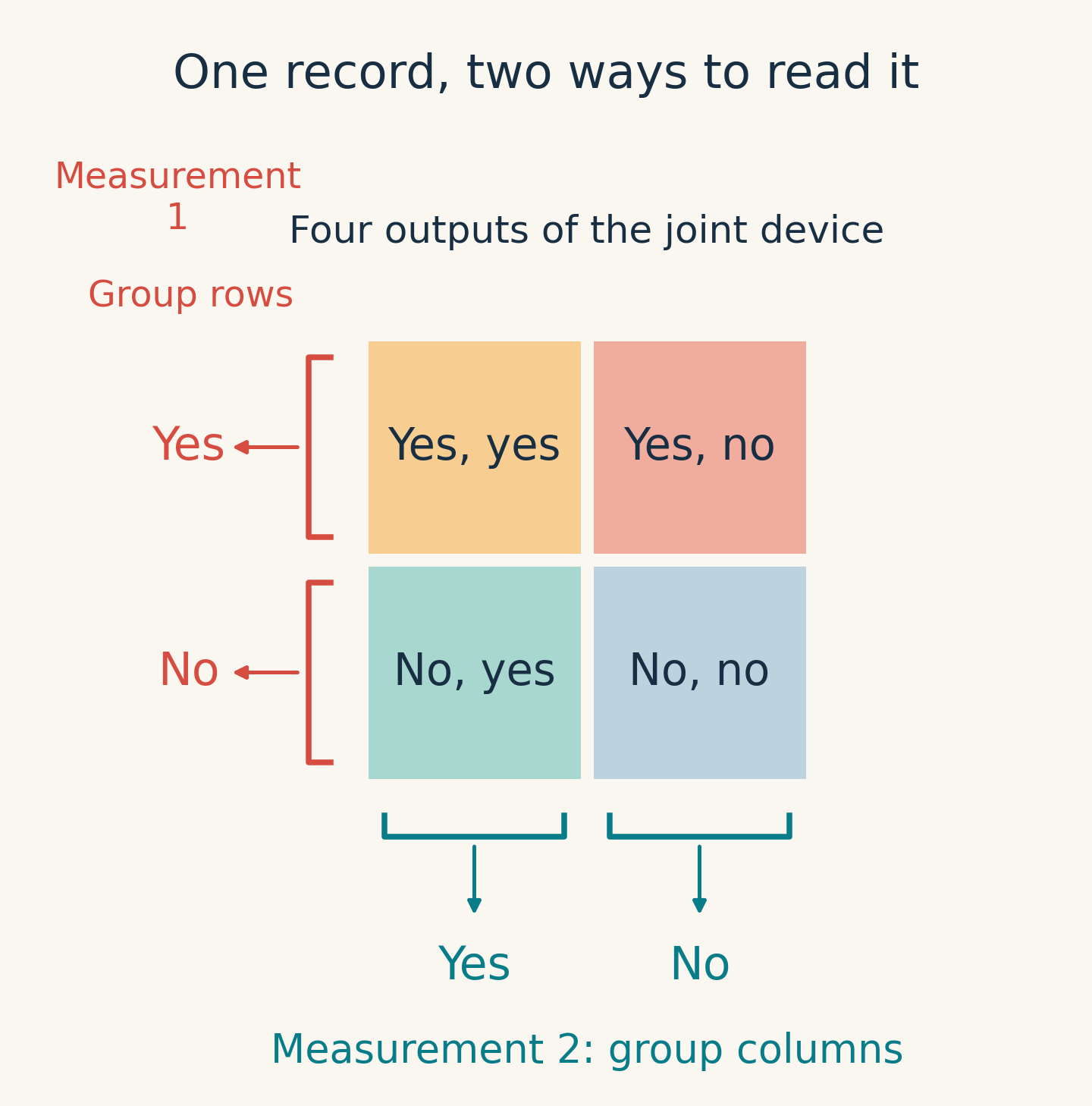
Why is this distinction worth counting? If two measurements are compatible, the choice of measurement can be postponed until after the joint record has been obtained: all that is needed is a different grouping. If they are incompatible, this way of reading a record cannot replace the measurement choice. In quantum information research, incompatibility is therefore a resource: it can support certain tasks involving quantum correlations or the discrimination of quantum states. Having this resource, however, does not mean that any combination of devices or any experiment will automatically gain an advantage.

Ideal spin measurements make up only a small fraction of all measurements. The devices we can consider may also have noise, give less distinct readings, or even favor one output. These changes can make previously incompatible measurements compatible. Thus, examples involving two ideal measurements cannot answer the question, “If we randomly pick two measurements, how likely are they to be incompatible?”

First define what “random” covers

A qubit is the simplest unit of quantum information; it can be carried by an electron’s spin or a photon’s polarization. For a qubit, a measurement with just two outcomes can be described by one real number and one three-dimensional arrow.

The arrow’s direction specifies the direction of the quantum states that the measurement distinguishes. Its length indicates how sensitive the measurement is to these differences, a property usually called “sharpness.” In the absence of outcome bias, the maximum length corresponds to an ideal measurement. Shortening the arrow makes the two outcomes less informative about differences between input states. When the arrow has zero length, the device’s output probabilities are entirely independent of the input state, just as if it were tossing a possibly biased coin.

The additional real number describes outcome bias. Once the positive and negative labels have been chosen, we denote it by $a_0$, ranging from $-1$ to $1$. When the input is the maximally mixed state—a quantum state that can be understood as favoring no direction—the probabilities of the two outputs are $(1-a_0)/2$ and $(1+a_0)/2$, respectively. Thus, $a_0=0$ is called unbiased; this does not mean that the device gives equally probable answers for every input state.

These parameters cannot be combined arbitrarily. If we denote the arrow by $\mathbf{a}$, a valid measurement must satisfy

$$\|\mathbf{a}\|\leq 1-|a_0|$$

Here, $\|\mathbf{a}\|$ is the arrow’s length, and $|a_0|$ is the magnitude of the bias. The greater the bias, the shorter the maximum permitted arrow. At a fixed bias, all allowed arrows fill a three-dimensional ball. As the bias approaches either end of its range, the ball shrinks to a point, and the device always gives the same answer.

This study treats the real number and the arrow’s three components together as four-dimensional coordinates. It samples uniformly over the entire valid region using ordinary Euclidean volume, then draws the second measurement independently. “Uniform” means that small four-dimensional pieces of equal volume have equal chances of being selected. This is not equivalent to first choosing a bias uniformly and then choosing an arrow uniformly: the closer the bias is to either end, the smaller the volume of the allowed ball, and the less often that bias occurs in sampling over the whole region.

Only with this convention does the question have a unique numerical answer. For sampling restricted to unbiased measurements, a 2019 study by Lin Zhang, Hua Xiang, Xianqing Li-Jost, and Shao-Ming Fei had already found an incompatibility probability of $3/5$. When bias was allowed to vary, their numerical calculations gave a result close to $1/4$, leading them to conjecture that it was exactly $1/4$. Original study

In the present paper, Gewu researchers prove that, under the same sampling over the full parameter domain, the exact probability is actually

$$P_{\mathrm{inc}}=\frac{2}{5}-\frac{8\pi^2}{525} \approx 0.2496060282$$

$P_{\mathrm{inc}}$ denotes the probability that a random measurement pair is incompatible. It is about $0.0394$ percentage points below one quarter: among ten thousand sampled pairs, about 2,496 would be incompatible on average, rather than 2,500. This is a conversion of the probability, not an observed result from ten thousand experiments.

Such a tiny difference cannot be explained simply by adding decimal places. The real question is how to account for every measurement pair and prove that no small region has been missed.

From eight parameters to an angular window

Each of the two measurements has four parameters, making eight dimensions in total. Existing compatibility criteria can assess a particular pair of measurements, but they do not directly tell us how much volume is occupied by the region that satisfies—or fails to satisfy—the criterion.

First, remove an irrelevant complication: rotating both arrows together does not change whether they are compatible. Their absolute orientation does not matter; their relative angle does. Once the biases and arrow lengths are fixed, we therefore need only ask which angles lead to incompatibility.

Unbiased measurements offer an intuitive example. Take two arrows whose lengths are both 80 percent of the maximum. When the arrows coincide, the measurements are identical and naturally compatible. Turn them to a right angle, however, and they become incompatible. Keep turning until they point in opposite directions, and swapping the answer labels makes them equivalent to the same measurement again, restoring compatibility. In other words, incompatibility occupies only an intermediate range of angles.

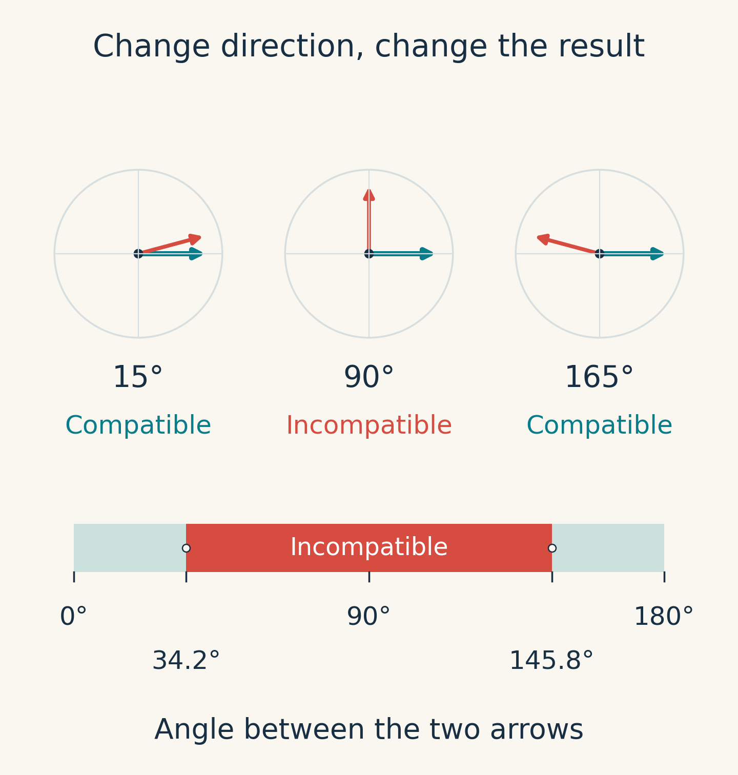
Random directions do not make every angle equally likely, either: more directions on a sphere lie near a right angle. One useful fact for the calculation is that, if the directions of the two arrows are each uniformly distributed over the sphere, the cosine of their angle is uniformly distributed between $-1$ and $1$. The cosine can be understood as a measure of alignment: it is $1$ for arrows pointing the same way, $0$ for perpendicular arrows, and $-1$ for opposite arrows. The incompatibility probability can therefore be calculated from the length occupied by the window on this “alignment” scale.

With bias, the window generally shifts away from the center of the scale, and whether a window exists at all depends on the other parameters. The key step taken by the Gewu researchers was to switch to coordinates that encode both bias and sharpness, simplifying the complicated square roots in the criterion. In the new coordinates, the region in which incompatibility can occur is defined by a simple circular-arc condition. Outside that region, all angles are compatible; inside it, each set of parameters is weighted by the window’s width.

The original eight-dimensional volume thus becomes a fourfold integral: the contribution of all directions has already been absorbed into the window width. What remains is to add up the windows for different biases and sharpnesses, using the volume weights of the original sampling scheme. Reparameterization neither changes the sampling nor discards measurements that are difficult to handle. It simply makes the boundary and weights amenable to exact treatment. The paper then reduces this integral to a one-dimensional integral and evaluates the endpoints using expressions that can be checked by differentiation, term by term, obtaining the answer containing $\pi^2$.

There is also a shorter check that suffices to rule out one quarter. The paper writes the same probability as an initial value minus a series of strictly positive correction terms. The initial value is about $0.270899$; after subtracting the first term, it is still about $0.251198$; after subtracting the second, it has already fallen to

$$\frac{5910272}{23648625}<\frac{1}{4}$$

More positive numbers remain to be subtracted, so the final value can only be smaller. This step can be carried out entirely with fraction arithmetic, without trusting the last few digits of floating-point integration. The geometry determines which measurements to count; this upper bound guarantees that the answer is close to one quarter but cannot equal it.

How favoring one answer erases incompatibility

The overall probability compresses the whole set of measurements into a single number. But it does not yet answer which measurements most readily lose their incompatibility.

Suppose the bias magnitudes of the two measurements are $u$ and $v$, both between $0$ and $1$. Fix these two values, then sample uniformly within their respective allowed arrow balls to obtain the conditional probability $p(u,v)$. The Gewu researchers prove that this probability does not increase as either bias grows, and that it has an exact boundary:

$$u+v\geq1\quad\Longrightarrow\quad p(u,v)=0$$

This result has a practical interpretation. Start with an unbiased two-outcome measurement and retain its original physical process, but change the rule for reporting the result: whenever the device reports “yes,” change it to “no” with probability $u$; leave an original “no” unchanged. The resulting measurement has bias magnitude exactly $u$, and its arrow shrinks to $1-u$ times its original length. To change the sign of the bias, simply swap the output labels. Thus, every biased measurement within the allowed range can be obtained in this way from some unbiased measurement.

If the two original measurements already have a joint record, both answers can be modified directly on that record. A compatible measurement pair cannot become incompatible through this rewriting of answers. Progressively rewriting the same collection of unbiased measurements in this way also produces exactly uniform samples on each slice of fixed bias. This explains why the conditional probability decreases monotonically.

More interestingly, when $u+v\geq1$, a joint device can be constructed directly. With probability $1-u$, let it perform the first original measurement and record “first measurement’s result, no.” With probability $1-v$, let it perform the second original measurement and record “no, second measurement’s result.” With the remaining probability $u+v-1$, let it measure nothing and simply record “no, no.” The probabilities of these three branches are nonnegative and sum to exactly $1$.

Reading only the first answer, we find that the device actually performs the first measurement with probability $1-u$ and otherwise always reports “no.” This is exactly the rewriting rule for bias $u$. The same reasoning applies to the second answer. Thus, a measurement following a single random choice does indeed recover the statistics of both biased measurements. The seemingly abstract threshold simply says that “the probabilities of performing the two original measurements add up to no more than one.”

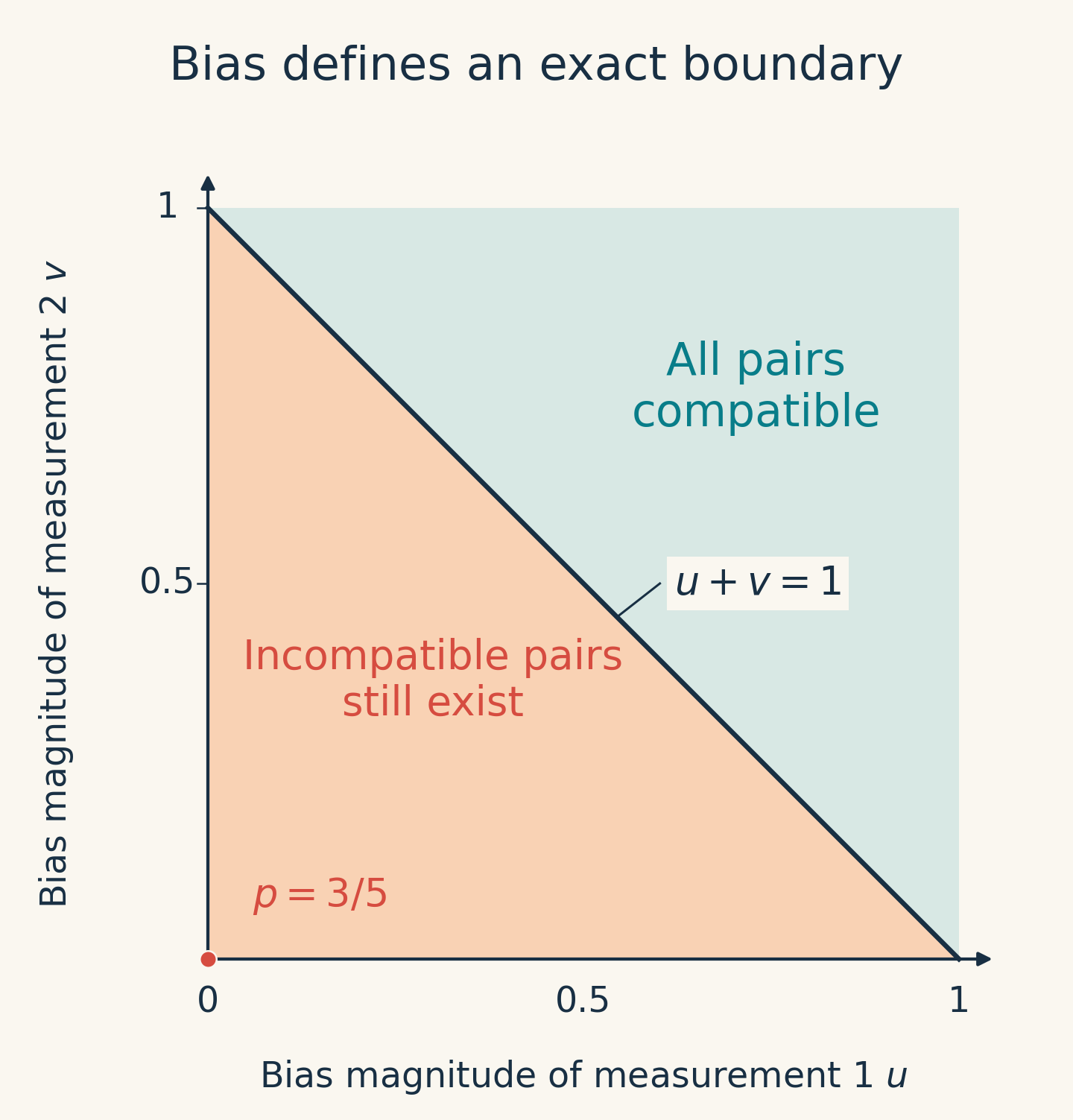
When $u+v<1$, the Gewu researchers prove that a region of incompatible measurement pairs with nonzero volume always remains. This clarifies the meaning of both sides of the boundary: it precisely separates “incompatibility is still possible” from “compatibility is guaranteed,” rather than merely providing a conservative safety margin.

There is a finer distinction near the boundary. Away from its two endpoints, let $1-u-v$ denote how far the sum of the biases falls short of the boundary. The incompatibility probability approaches zero as the fifth power of this difference. Along a coordinate axis toward an endpoint, however, it vanishes linearly. These are asymptotic laws near the boundary and cannot be applied across the entire diagram. They show that, even once the overall probability is known, the way incompatibility recedes through measurement space has a structure of its own.

The proportion obtained in this work has a clearly defined scope: qubits, two measurements with two outcomes each, and Euclidean uniform sampling over the specified parameter domain. A different sampling scheme can change the probability. The monotonicity under output rewriting and the joint-device construction above also apply to quantum systems of higher dimension; the full probability and regional structure in higher dimensions remain unresolved by this study.

What matters more than “how much less than a quarter” is therefore when that joint record can exist. Different directions can make two measurements impose demands that cannot both be met, while blurring and bias weaken those demands. The exact calculation turns this tension into a verifiable proportion. The bias boundary goes further, telling us how much information must be erased before the conflict between quantum measurements can always be accommodated in a single record.

---

Research source: The present paper, The incompatibility probability of random binary qubit measurements: exact value, fixed-bias phase diagram, and critical laws at the boundary. This article reports mathematical results; it contains no new experimental data. For the definition of unbiased measurements and the joint implementation of noisy spin measurements, see the original study by Grinko and Uola. All illustrations were created specifically for this article.