Periodic neural coding: how fast can it pinpoint a location?

A group of neurons can encode many locations with distinct activity patterns, yet the patterns at two distant places may differ in just one cell. Detecting that difference through random spikes takes time. How should a limited number of cells be allocated to balance spatial resolution and discrimination speed? In an idealized model of periodic coding, Gewu researchers have established a speed limit that no design can escape.

After an animal travels some distance, the same neuron becomes active again. This is nothing unusual in the brain's positioning system. In 2005, Torkel Hafting, Marianne Fyhn and colleagues reported a type of cell in the rat entorhinal cortex that becomes active repeatedly as the animal reaches a series of regularly arranged locations. These locations form a triangular lattice in the plane, giving the cells their name: “grid cells.” A single cell's signal repeats; combining the activity of multiple cells offers a way to distinguish locations. Original study

Repetition has an appealing advantage: the same local pattern can extend over a larger space. But it also carries a risk. If two places are exactly one repeat period apart, the signal at that period alone cannot tell you which one you occupy. Adding denser patterns provides detail, but also makes repetition more frequent. For this way of representing position to be useful, we need to ask both how many locations it can distinguish and how long we must observe it to tell them apart.

Gewu researchers studied the latter question. The answer in their new paper applies to a strictly defined mathematical model: locations lie on a circular track, and cells have only two firing rates, high and low. The coarsest group has a period equal to a full circuit, while the periods of successive groups become shorter by integer factors; each cell fires at the high rate over one continuous interval within each period. By comparing all permitted cell arrangements, the paper determines how the best discrimination time varies with the required precision and the total number of cells. Accompanying paper

Two distant locations may differ in only one cell

First, straighten out the circular track, keeping its ends joined. Let the length of a full circuit be one. One model cell maintains a high firing rate over the first half of the circuit and a low rate over the second half; another cell repeats every half circuit, and a third every quarter circuit. Each of the latter two cells also maintains a high firing rate over half of its own period.

Represent high and low rates as light and dark, and we get three rows of bands. As we move along the track, we can read all three rows at once. Together, the three rows divide the circuit into eight segments, each with its own unique combination of light and dark: the coarse row distinguishes broad regions, while the fine row adds smaller distinctions.

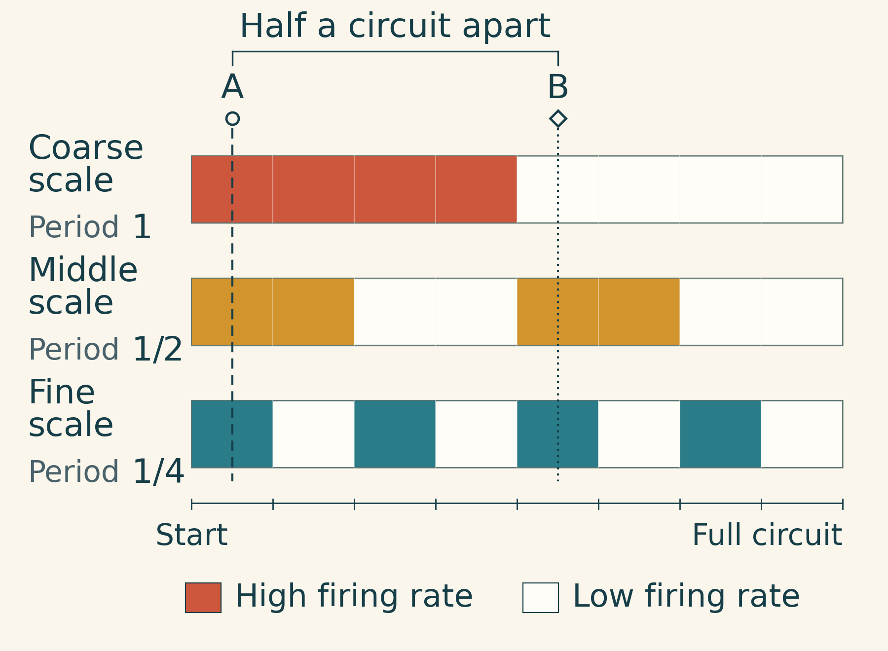
Very few cells can thus combine to produce many patterns. Yet consider locations A and B in the figure. They are half a circuit apart, and the second and third cells give exactly the same signals at both; only the first cell changes its firing rate. Even if we keep adding cells with shorter periods, they too will repeat at these two locations as long as their periods remain one-half, one-quarter, one-eighth, and so on, of a full circuit.

This shows that “many distinguishable patterns” and “every pair of patterns is easy to distinguish” are two different things. The latter depends on how many cells actually provide a difference.

The light and dark areas here depict firing rates; they are not lights that can be read with perfect accuracy at a glance. Neurons send out trains of spikes. As the statistical basis for this mathematical framework, Guilherme Ost and Patricia Reynaud-Bouret modeled the spike trains as independent, with spikes occurring randomly at fixed average rates. Over a short interval, a cell with a high firing rate may still emit few spikes, while one with a low rate may happen to emit more. Identifying a location therefore requires accumulating evidence. Statistical model and discrimination framework

If two locations give every cell the same firing rate, no amount of observation can distinguish them. If many cells have different firing rates at the two locations, more independent evidence is available and the required observation time can be shorter.

The paper reduces this relationship to a count. Compare two locations and count the cells that change from a high firing rate to a low one, then count those that change in the opposite direction; take the larger of the two counts and call it $\Delta$. With the high and low firing rates fixed and a sufficiently small permissible error rate fixed, the time needed for discrimination is of the same order as $1/\Delta$. The paper therefore directly defines the normalized discrimination time for a pair of locations as

$$T_{\mathrm{pair}}=\frac{1}{\Delta}.$$

Here, $T_{\mathrm{pair}}$ measures how hard the pair is to distinguish; if $\Delta=0$, it is set to infinity. This measure of time removes fixed multiplicative factors and cannot be read directly as a number of seconds.

Precision and speed share the same pool of cells

Next, we need to clarify what “best” means.

First, specify a distance requirement $\rho$, expressed as a fraction of the full circuit's length. We require only that two locations at least $\rho$ apart can be distinguished; closer locations may be left indistinguishable. Distance on the circle is the shorter of the two connecting arcs, so the maximum distance is half a circuit.

For a fixed code, find the pair with the longest discrimination time among all pairs that meet this requirement. This measures the code's worst-case performance. Then let the designer choose anew how many groups to use, how many cells to put in each group, the period of each group, and the interval over which each cell maintains its high firing rate, in search of the best arrangement. This problem—first evaluating the worst performance, then choosing the best design—is called a minimax problem.

The task here compares two known candidate locations: deciding from the spikes whether one is “at A or at B.” It is not equivalent to estimating an unknown coordinate anywhere along the track from spikes alone.

Gewu researchers prove that with $n$ cells in total, if the required distance is less than $2^{-n}$, every arrangement leaves some pairs that meet the distance requirement but cannot be distinguished. At $\rho=2^{-n}$, designs already exist that make every qualifying pair distinguishable. This resolution threshold was established in earlier work; the new paper fills in the best achievable speed from that threshold onward.

In the range $2^{-n}\leq\rho\leq1/2$, the best normalized discrimination time, $T_{\mathrm{opt}}$, satisfies

$$c\,\frac{\log_2(1/\rho)}{n} \leq T_{\mathrm{opt}}\leq C\,\frac{\log_2(1/\rho)}{n}.$$

Here, $c$ and $C$ are positive constants that do not vary with the number of cells or the precision requirement; $\log_2$ denotes the base-two logarithm. The two bounds do not yet give a single exact value, but they do pin down the order of the scaling.

Why does a logarithm appear? Halving a circuit three times takes us to one-eighth of a circuit; halving it six times takes us to one-sixty-fourth. $\log_2(1/\rho)$ is precisely the number of these successive halvings. The result shows that the order of the optimal time is determined by this measure of fineness divided by the total number of cells. The finer the requirement, the harder it is for a limited number of cells to guarantee rapid discrimination; with the precision requirement fixed, adding cells can speed it up.

An example with just six cells makes the trade-off concrete. In the first arrangement, each of the six cells is assigned one of six successively halved periods. This divides the circuit into sixty-four segments, yet some locations half a circuit apart still differ in only one cell. That weakness holds the normalized discrimination time at one.

In the second arrangement, only the three coarsest periods are retained, each assigned two cells with exactly the same active intervals. This distinguishes only eight segments, but gives every original cell difference two independent sources of spike evidence. For any two locations at least one-eighth of a circuit apart, the normalized discrimination time falls to one-half.

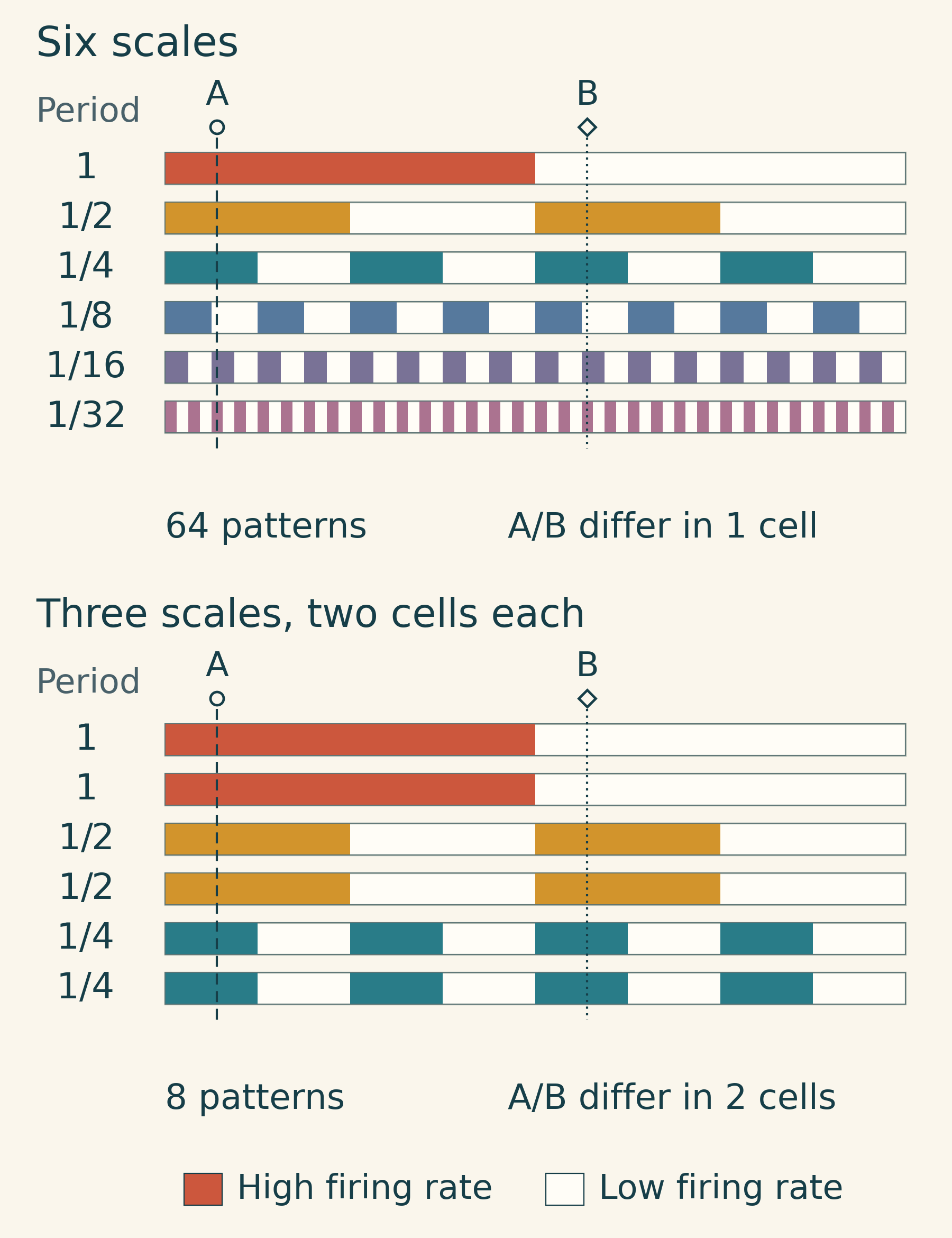
With the same number of cells, allocating them across more scales can buy finer resolution; using them to duplicate existing signals may instead speed up discrimination on coarser tasks. But this example compares only two arrangements. Could an uneven allocation of cells among groups, or periods that shrink by factors of three or five, outperform both?

Ost and Reynaud-Bouret had already provided some good designs, leaving this question open: how much faster can discrimination become if the entire structure is allowed to change? The key to the new paper is a constraint shared by every permitted design.

Weaknesses at every scale must be covered by cells

The proof starts with the same pair of locations half a circuit apart shown in Figure 1.

When a displacement is exactly equal to a cell's period, that cell gives the same signal at both locations. Because the model requires each larger period to be an integer multiple of the next smaller one, the finer groups repeat as well. The burden of distinguishing the two locations then falls on the coarser groups.

Changing the displacement to another period produces another such test. Even a design that is sensitive to one class of location pairs may expose a weakness at other scales. To distinguish even the worst-case pair quickly, a design must address all these tests at once; densely packing active intervals into a local region is not enough.

Earlier work had already expressed this as a lower bound for a fixed structure. But that bound involved the numbers of cells in the groups, their periods, and the precision requirement all at once. To compare every structure, it is not enough to calculate an answer for one set of parameters.

Gewu researchers used a finite-sum identity called “Abel summation.” It rewrites a sum as a weighted sum of partial sums. Here, each partial sum records the cells' contributions from the coarsest scale through a given level, while the weights come from differences between neighboring scales.

Crucially, all these weights are nonnegative. The minimum contribution needed at each level to avoid a weakness can therefore be substituted and summed without losing the constraint through cancellation of positive and negative terms. After rearrangement, the calculation still accounts for the same total cell budget. Making discrimination fast at every scale requires enough cells to meet all these demands together.

This calculation also constrains attempts to “skip scales.” A period can shrink by a large factor in one step, but the weight of the corresponding constraint then grows as well. By converting the ratios between successively shorter scales into logarithms, the proof accumulates the contributions at each level until only the total span from a full circuit to the target precision remains. No matter how many intermediate groups there are, or which scales receive extra cells, the budget requirement remains proportional to $\log_2(1/\rho)$. With the total cell count fixed, the difference count that can be guaranteed for every pair is at most a fixed multiple of $n/\log_2(1/\rho)$. Taking the reciprocal gives a lower bound on time that no permitted structure can beat.

The lower bound must also be matched by a design achieving the corresponding order; otherwise, it might be only a loose restriction. The other half of the paper comes from existing constructions: when enough cells are available, groups with successively halved periods, with cells distributed as evenly as possible and their high-rate intervals appropriately staggered, achieve the required order of speed. Near the resolution threshold, a fine-scale construction with one cell per group completes the coverage. Together, the two provide the upper bound.

The advance is thus from “one arrangement can do this” to “no other permitted arrangement can be arbitrarily faster in terms of scaling.” The speed cost of fine spatial resolution becomes a property of this entire class of models.

Optimal for one task does not mean optimal for every task

The answer still leaves a question of particular relevance to the brain. The paper allows the entire code to be chosen anew for different distance requirements. It does not prove that a single fixed cell structure can simultaneously achieve the respective optimal speeds for many precision requirements.

Distinguishing the two ends of a road and detecting a tiny movement at one's feet require different levels of precision. If the position signals have to be rebuilt each time, optimality for an individual task may say little about efficiency in practice. Answering this question will require either finding a code that works across multiple distance requirements or proving that no such code can exist.

Real grid cells also lie outside this paper's assumptions: their activity does not follow neat high–low steps, space has more than one dimension, and different periods need not be strictly nested by integer factors. The paper does not prove that real brains reach this bound, nor does it give animals' reaction times. It offers a theoretical benchmark with clearly defined limits; the paper also states that its results await further validation by experts in the field.

Return to those two distant locations that differ in only one cell. Fine spatial patterns can create many distinct addresses without necessarily leaving enough clues to tell every pair apart. This study brings both demands into the same budget: cells must represent the details of position while also providing a sufficiently quick answer where locations are hardest to distinguish.

---

This article is based on the accompanying paper, “The Minimax Discrimination Rate of General One-Dimensional Periodic Grid Codes.” The cover and article figures are all original programmatically generated artwork; the article figures are model schematics and small-scale exact calculations. Drawing source files and verification notes are supplied with the article.