The Other Half of Quantum Correlations Raises the Cost of Classical Simulation

Two sets of quantum experimental records exceed the limit allowed by classical theory by exactly the same amount. Must they be equally difficult for a classical model to simulate? A theoretical study of multipartite entanglement finds that the answer can be no: the test commonly used here examines only half the measurement combinations, while the other half contains additional constraints. Once those combinations are included, a classical model sometimes has to link hidden information more tightly to measurement choices to reproduce all the results.

This involves a condition in Bell tests that can easily recede into the background. Imagine several experimental stations far apart. Each receives a particle, chooses how to measure it, and then compares its results with the others. A classical explanation might hold that the particles carry information that has not yet been observed, determining how they respond to different measurements. This information is called hidden variables. If each station can respond only on the basis of its local measurement choice and the hidden variables, and if the measurement choices are statistically independent of those variables, the correlations between outcomes cannot exceed the bound set by a Bell inequality.

Quantum mechanics permits correlations beyond that bound. But if we retain the requirement that each station responds locally while relaxing the independence of measurement choices from hidden variables, a classical model may once again be able to simulate the quantum statistics. The question then shifts from “Can it be simulated?” to “How much independence must be given up, at a minimum?” The cost here means the extent of that relaxation, not how long a computer must run or how much the equipment costs.

Establishing this minimum helps us understand precisely which classical explanations a Bell-test record rules out. The amount by which a test exceeds the classical bound may not fully capture this requirement. In this paper, Gewu researchers derive the exact minimum cost of reproducing every outcome probability for specified measurements on a class of entangled systems with at least three particles. The case of an even number of particles exposes the limitations of a single test score particularly clearly.

How a Classical Model Can “Pick Its Answers”

Restrict each station to two measurements, denoted $X$ and $Y$. These are two standard qubit measurements, corresponding to mutually perpendicular directions in the representation of a quantum state; each yields only $+1$ or $-1$. With four stations each choosing one measurement, there are sixteen joint settings, such as $XXXX$ or $YXXX$. A letter’s position identifies the station.

A local classical model can specify two answers in advance for each station: what to output when $X$ is chosen, and what to output when $Y$ is chosen. Together, all the stations’ answers make up a “response table.” The hidden variable identifies which table to use. Even if the model originally allows random responses, the extra random numbers can be incorporated into the hidden variable. Describing the model through preset answers therefore does not exclude general local models.

Measurement independence requires the probability of encountering each response table to be the same for every joint setting. Allow measurement dependence, and this changes: certain tables may appear more often when the setting is $XXXX$; switch to $YXXX$, and other tables may receive more weight. Each station still answers according to its own table, but the composition of the ensemble of tables is now correlated with the joint setting. This description specifies only a statistical relationship, not the physical mechanism that produces it.

How can we measure the difference between two ensembles of response tables? We can ask how much probability must be moved, at a minimum, to turn one distribution into the other. Mathematically, this is called the total variation distance. Suppose, for example, that one category of tables accounts for 40 percent of the first distribution and 20 percent of the second. If the entire 20-percentage-point reduction is transferred to another category, with everything else unchanged, the distance is $0.2$.

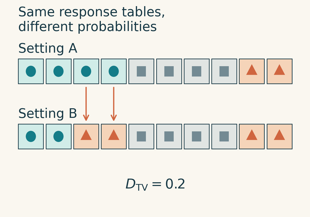
For a given model, the paper compares every pair of joint settings and denotes the largest total variation distance by $F$. If $F=0$, one fixed distribution can serve every setting, and measurement independence is fully preserved. We must then find the smallest $F$ among all local models capable of reproducing the target statistics. That is the minimum cost discussed here.

This number cannot be read directly as “how many experimental trials were manipulated,” nor does it measure human free will. It has a more specific statistical meaning: take two settings whose distance attains $F$, and let them occur with equal probability. Given knowledge of the hidden variable, an optimal guesser can distinguish between the two settings with a success probability of $(1+F)/2$. Identical distributions offer no basis for guessing; differences between them provide clues.

One Type of Measurement Reveals One Coherence Component

The systems examined in the paper are based on GHZ states. Named after Greenberger, Horne, and Zeilinger, these are a class of multipartite entangled states. If we call each qubit’s two basis states zero and one, an ideal GHZ state coherently superposes “all qubits are zero” and “all qubits are one.”

“Coherently” is the key word. If we simply toss a coin and sometimes prepare all zeros and sometimes all ones, the two preparations form only a classical probabilistic mixture. A coherent superposition also retains the relative phase between the two possibilities. With suitable measurements, this relationship can produce interference, changing the statistics of the joint outcomes.

The Gewu researchers allow this coherence to weaken and its phase to change, but the quantum state remains confined to the subspace spanned by the all-zero and all-one states. In other words, this is a precisely defined family of states, not one that encompasses every kind of laboratory noise.

To observe this relationship, multiply the outcomes from all stations in a single measurement trial, then average over many trials. This average is called the full correlation, denoted $E$: if the product is always $+1$, the average is $+1$; if positive and negative products occur equally often, it is zero. The quantum states considered here have a particular property: if we multiply the outcomes from any proper subset of stations, the average is zero. The differences are concentrated in the product involving all stations together.

With the $X/Y$ directions fixed, the complete measurement table splits into two halves. One half consists of settings with an even number of $Y$ measurements; the other consists of settings with an odd number of $Y$ measurements. The two groups probe two coherence components, denoted $c_0$ and $c_1$ in the paper, which mathematically correspond to the real and imaginary parts of the coherence. They can be understood as two components of the same coherence relative to the measurement directions. Looking at one alone does not determine the other.

For four particles, the full correlation for $XXXX$ is $c_0$; combinations containing two $Y$ measurements give $-c_0$; and $YYYY$ returns to $c_0$. The odd group behaves differently: combinations with one $Y$ measure $c_1$, while those with three $Y$ measurements give $-c_1$.

The even-group Mermin test discussed here adds the correlations in the first group with these signs and compares the sum with the classical bound. The resulting score depends only on $c_0$. However $c_1$ changes, the entire probability table for the even group can remain unchanged. The missing information has therefore not merely been averaged away: these measurements never probed the other coherence component in the first place.

This question connects closely with earlier research. Aaron Alai’s work derived the minimum cost for ideal GHZ states under these even-group settings, verified it for up to thirteen particles, and proposed a rule extending it to any number of particles. The Gewu researchers prove that rule, extend the treatment to weakened coherence, and include the odd-group settings in the same optimization problem.

Identical Records, Different Minimum Costs

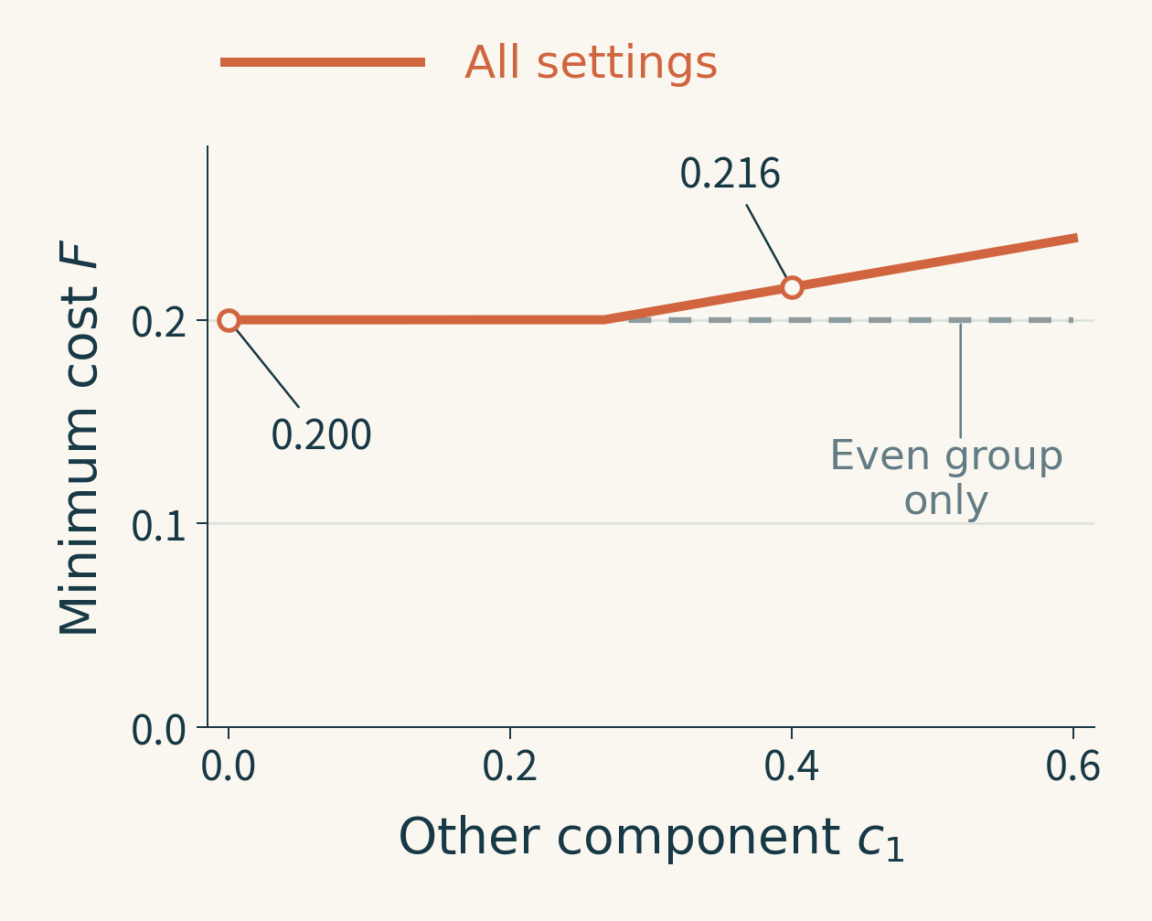
Consider two four-particle states. In both, the all-zero and all-one basis states each have a population of one half, and $c_0=0.8$. In the first, the other component is $c_1=0$; in the second, it is $c_1=0.4$. Both are allowed quantum states.

With only even-group measurements, the two states are completely indistinguishable: for every setting, the probability of every outcome string is the same. Their Mermin scores are also identical, both $1.6$ times the classical bound and thus already exhibiting a Bell violation.

Once the odd group is included, however, the first state has zero full correlation for all those settings, whereas the second has full correlations of $+0.4$ or $-0.4$. The paper proves that reproducing all sixteen settings for the first state has a minimum cost of $0.200$. Reproducing the second requires at least $0.216$, and a local model attaining that value does exist.

The difference is small, but exact. The first model is already sufficient to reproduce an even-group record that exceeds the classical bound. Adding the odd-group record of the second state nevertheless imposes a higher requirement.

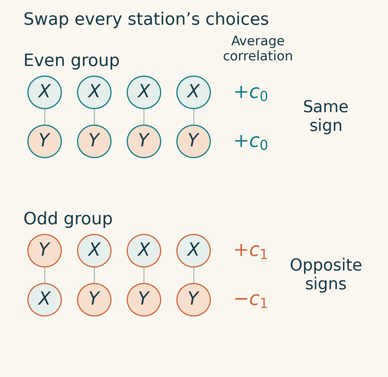
Why does an additional cost arise? Consider the constraints on a fixed response table. Swap the choices at all four stations: $XXXX$ becomes $YYYY$, and $YXXX$ becomes $XYYY$. Two settings related in this way are called complementary settings.

For a classical response table, first calculate the product of the four answers for $XXXX$, then multiply it by the product of the four answers for $YYYY$. This amounts to multiplying together every station’s $X$ and $Y$ answers once each. Using $YXXX$ and $XYYY$ instead still multiplies the same eight answers once each. For any given table, then, the relationship between the two products must be the same in both pairs: either the products have the same sign in both pairs, or they have opposite signs in both.

The sign pattern of the quantum correlations imposes different requirements. When $c_0$ and $c_1$ are both positive, the average correlations for $XXXX$ and $YYYY$ are both positive, whereas those for $YXXX$ and $XYYY$ have opposite signs.

When correlations are imperfect, response tables can be mixed; not every table has to match the signs of the target averages. But an ensemble of tables serving both groups of settings is still constrained by the shared structure just described. The paper finds that, for an even number of particles, once the second component becomes strong enough, the changes in distributions prepared for the first component alone may no longer suffice. The distributions for different settings must move further apart. This additional cost comes from the joint requirement, while the even-group Mermin score remains entirely unchanged.

This is not a universal rule that “measuring more always costs more.” The plateau in Figure 2 shows that adding a weaker component may initially carry no extra charge. For an odd number of particles, the result is different again: within the states and measurements specified in the paper, the full cost is determined solely by whichever component has the larger absolute value; the weaker component adds no further cost. In this case, swapping all $X$ and $Y$ measurements exchanges the odd and even groups, changing their shared structure. The approach in the paper is to first construct an optimal model with equally strong components, then introduce random sign flips independent of the setting to weaken only one component. This preserves local responses without increasing the distances between distributions. The weaker component can therefore be obtained for free.

How to Know the Minimum Has Been Reached

Finding a classical model with a low cost proves only that “this much is sufficient,” not that “no less is possible.” The paper establishes its result from two directions: explicitly constructing models while deriving a lower bound for every possible local model, and finally making the two meet.

One simplification follows Alai’s approach. The analysis initially needs to consider only what response tables predict for the full product, grouping tables with exactly the same predictions into a single class. This may sound as though the individual stations’ outcomes have been discarded, but they can be restored: uniform randomization within a class is equivalent to randomly flipping the answers of an even number of stations. The full product is unchanged, while for any nonempty proper subset of stations, positive and negative products cancel after randomization.

This exactly restores the target quantum states’ zero correlations for subsets of stations. Crucially, the same randomization rule is applied to every setting, so it does not increase the total variation distance. The cost achieved in reproducing the full-product statistics can therefore also reproduce the probability of every complete outcome string, rather than just an aggregate score.

Building on this simplification, the Gewu researchers use the structure of the response tables and target sign patterns to construct different probability mixtures. For even numbers of particles, they also compare the differences between distributions for many pairs of settings. If classical tables are to satisfy the correlations of both groups simultaneously, a weighted sum of these distribution differences cannot be too small; yet it cannot exceed the model’s maximum total variation distance. This yields an unavoidable lower bound. The explicitly constructed models attain that bound exactly, making “minimum” a proven conclusion.

The researchers did not conduct experiments with increasing numbers of particles and then extrapolate a trend. The paper’s conclusions are analytic and cover any number of particles from three upward. Numerical optimization for smaller systems helped identify the constructions but does not supply the proof.

This also shows that the size of a Bell violation and the minimum cost considered here are not the same measure. Take an ideal GHZ state with coherence components $(1,0)$. The ratio of its even-group Bell score to the classical bound grows exponentially with particle number, yet the minimum cost for the complete measurement set always remains below $1/2$ and gradually approaches it. A larger violation cannot be directly translated into a proportional increase in measurement dependence.

From Exact Answers to Experimental Records

Real experiments need not fall within this family of GHZ states. A Mermin score therefore cannot simply be plugged in to claim an exact cost. But one joint constraint in the paper can be applied directly to measured full correlations for even numbers of particles, without first fitting the quantum state to a GHZ model. For general data, it gives a lower bound on the minimum cost; exact equality requires additional conditions.

A finite number of trials also introduces statistical fluctuations. The Gewu researchers propose sampling the odd and even groups of settings with predetermined probabilities and recording only one sign-corrected full product per trial. After subtracting the statistical error allowance, this yields a lower bound on measurement dependence with a confidence guarantee. The devices may remember the past and drift over time. What is inferred, however, is the degree of dependence in each trial conditional on the preceding record, averaged over trials—not a requirement that every trial meet the same minimum value.

This scheme also relies on explicit conditions for generating the inputs: both the random sampling within each group and the deviation of actual choice probabilities from their design values must be controlled. Aggregate setting frequencies that match expectations do not by themselves guarantee that these conditions hold trial by trial. Input biases can also inflate the score and must be separately calibrated and subtracted. These are theoretical methods of analysis proposed in the paper, not an experimental demonstration already carried out. Nonorthogonal measurements, detection losses, and other types of entangled states require new results.

Return to the two records at the beginning. They exceed the classical bound by the same amount, yet impose different requirements on classical alternative explanations. To determine how tightly a model that preserves locality must link hidden information to measurement choices, we need to ask which outcomes it must reproduce. For these multipartite systems, the omitted half of the measurements can reveal different constraints behind the same test score.

---

Research source: Minimal Measurement Dependence Required to Simulate GHZ Correlations, available in the accompanying paper.pdf. The main results are Eqs. (11)–(14); the four-particle comparison is in “Physical consequences”; proofs are in Appendices A–C; finite-sample analysis and input calibration are in Appendices D–F. The illustrations and theoretical curves in this article are original programmatically drawn graphics, with source code in sources/.