A Gas’s Chances of Running Backward Are Written in Its Entropy Increase

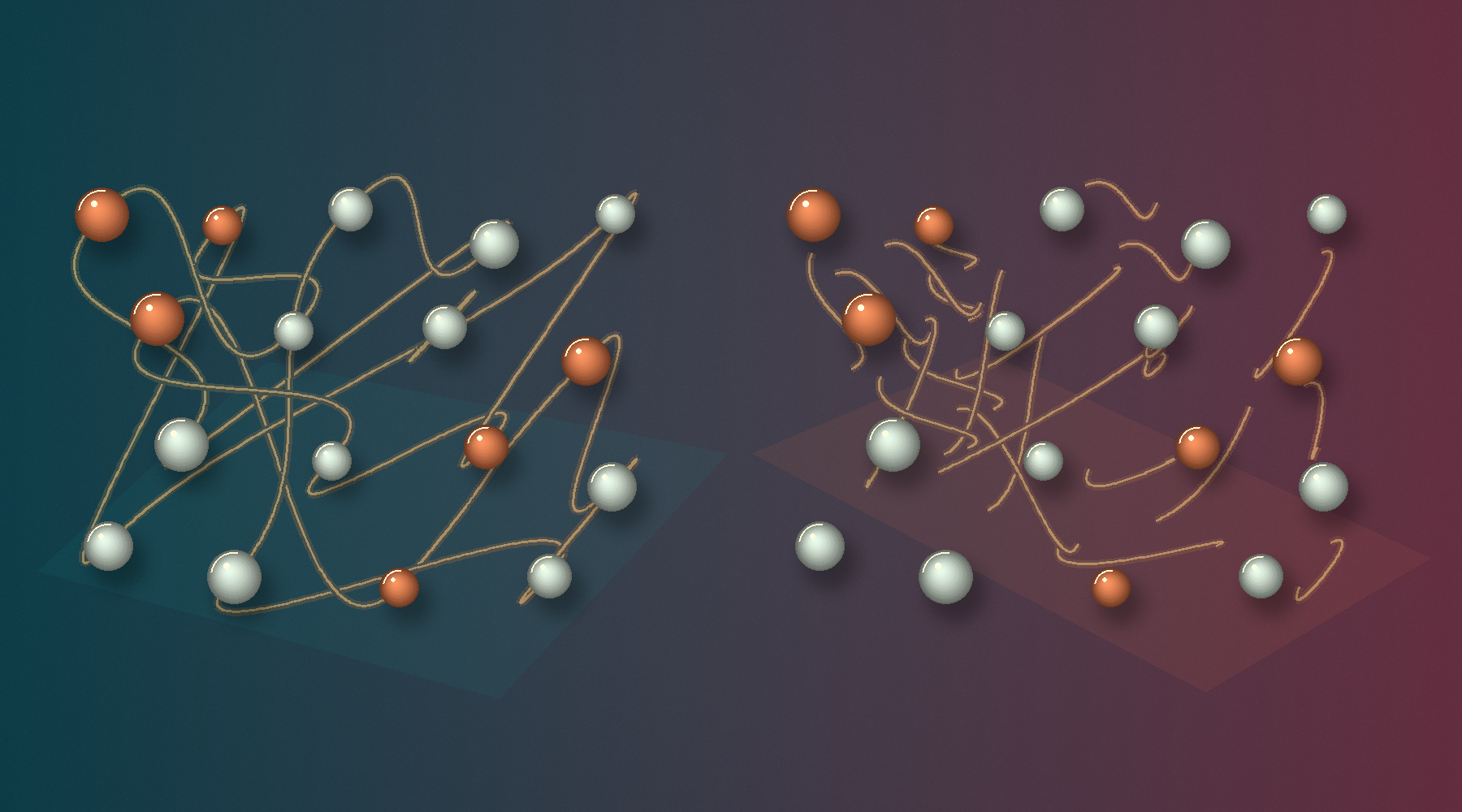
Reverse every particle’s velocity simultaneously in a gas whose particles are colliding, and the gas will retrace its path. But if we prepare another gas using only the position and velocity statistics at that instant, how likely is it to look as though it, too, is running backward? The two gases can have the same single-particle statistics, yet their futures depend on correlations between particles that those statistics do not record. In a dilute hard-sphere model, a researcher at GeWu has expressed this difference as a probability exponent: the greater the preceding entropy increase, the harder it is for the newly prepared gas to pass a specified time-reversal test.

The same statistics, different pasts

First imagine a collection of small spheres that undergo elastic collisions only when they touch. There is no friction, and no energy is lost in collisions; between collisions, the spheres travel in straight lines. If all their velocities are reversed exactly, a pair of spheres that previously collided and moved apart will approach each other again and undergo the reverse collision. This is the heart of Loschmidt’s reversibility problem: if the microscopic rules allow both forward and backward motion, why does the everyday behavior of a gas have such a clear direction in time?

When describing a gas, we do not usually list the positions and velocities of all its spheres. Instead, we ask: if we pick one particle at random, what is the probability that it lies within a particular range of positions and has a particular velocity? Bringing these probabilities together gives the single-particle distribution. It includes both position and velocity, making it far more detailed than a few numbers such as temperature and pressure, but it still does not tell us how each particle’s state fits together with those of the others.

“Correlation” has a specific meaning here: knowing one particle’s state changes our assessment of the states of other particles. Collisions establish just such relationships. After two spheres collide, their velocities are subject to shared constraints from the conservation of energy and momentum. Each then collides with other spheres, drawing more particles into these relationships. The single-particle distribution retains the changes in velocity statistics, but does not retain an itemized record of these shared constraints.

So taking a statistical “snapshot” of the exactly reversed gas and then sampling particle states from that snapshot does not reproduce the original gas. The original retains correlations generated by its earlier evolution. The newly prepared gas obeys only the specified single-particle distribution and the requirement that spheres must not overlap. It is under no requirement to retain the same relationships left by the collision history.

This also explains why identical single-particle distributions alone do not imply that the two gases must subsequently undergo the same macroscopic changes. Earlier work on hard-sphere limits by Thierry Bodineau, Isabelle Gallagher, Laure Saint-Raymond, and Sergio Simonella showed how details of initial correlations can affect the direction of time. The distinction between the two preparations has deep theoretical roots. “One-sided convergence in the Boltzmann-Grad limit”

The researcher at GeWu asks a more quantitative question: given a test that a genuinely reversed gas almost always passes, just how small is the probability that the newly prepared gas passes it by chance?

Entropy increase does not erase microscopic information

The Boltzmann equation uses the single-particle distribution to track how a gas changes over time. For suitable isolated gases, one of its central conclusions is that the entropy calculated from this distribution does not decrease. For now, we can think of this entropy as the amount of uncertainty in a statistical description that considers only one sphere’s position and velocity. Collisions change how velocities are distributed, and this uncertainty can grow.

The conclusion is different, however, if we record the joint probability distribution of the entire gas. Hard-sphere dynamics carries microscopic states into one another in a one-to-one fashion, preserving the volume they occupy in phase space. Phase space is simply the space that lists all the particles’ positions and velocities together. Under this evolution, the fine-grained entropy calculated from the full distribution remains constant.

There is no contradiction. The difference between the entropy obtained by treating the particles as independent and the entropy of their joint distribution measures their collective correlations. Looking at just one particle makes more possibilities seem available, because the description leaves out constraints on which particle states can occur together. Single-particle entropy can therefore increase while the entropy of the full distribution remains unchanged.

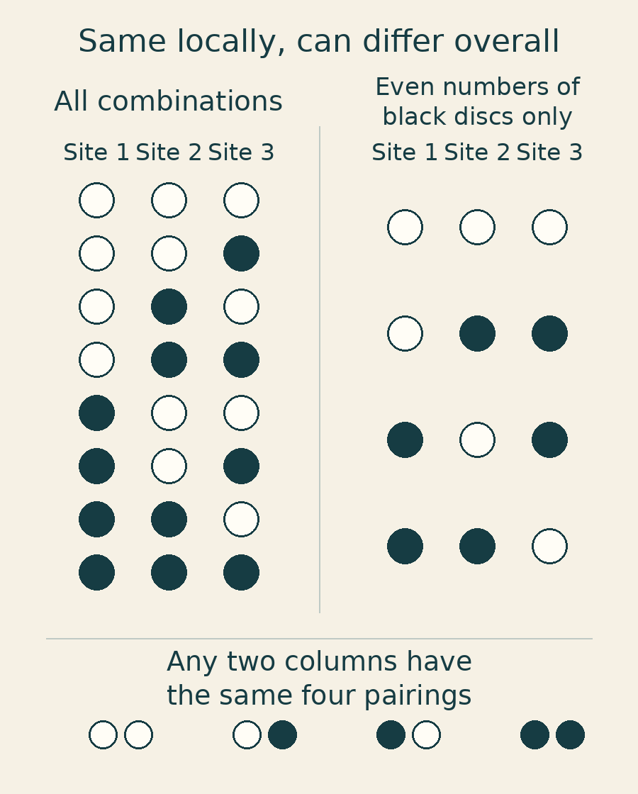
A small example illustrates the distinction. Place a black or white disc at each of three sites. The first preparation allows all eight combinations, each equally likely. The second allows only the four combinations with an even number of black discs, again each equally likely. At any one site, black and white each have probability one-half under both preparations. Even at any two sites, each of the four black-and-white pairings has probability one-quarter. But looking at all three sites at once reveals that the second preparation allows only half the combinations. Its constraint lies in the joint relationship among all three.

A real gas has far more possible states than these discs. To prove that this information accounting still holds in the passage from the microscopic model to the Boltzmann equation requires handling a difficult limit: the spheres become ever smaller and more numerous, and the fraction of space they occupy tends to zero, while the scale on which each particle undergoes collisions remains finite. This is the Boltzmann–Grad limit. It makes the gas sufficiently dilute without also removing the effects of collisions.

Yu Deng, Zaher Hani, and Xiao Ma previously proved that, over a time interval in which the solution of the Boltzmann equation exists and satisfies the prescribed bounds, the statistics of a few particles in a suitably prepared hard-sphere gas can approach the Boltzmann description. This result provides a mathematical bridge from reversible collision rules to the single-particle equation. It also supplies the underlying estimates needed for the present study. The original paper by Deng, Hani, and Ma, version 3

But closeness of distributions does not automatically imply closeness of entropies: very rare states can still contribute a non-negligible amount to the entropy calculation. The researcher at GeWu needed additional control over collision histories and the contributions of these rare parts of the distribution to the information content to carry the information accounting through this limit.

The result is that, under the paper’s preparation procedure, the collective correlation information divided by the mean particle number approaches the preceding increase in single-particle entropy. At the same time, if just two particles are selected using the paper’s sampling procedure, the average mutual information between them tends to zero. This does not mean that all the particles are independent, just as in the disc example, where the statistics of two columns are completely independent but all three columns obey a shared rule. The paper also proves that, under the corresponding sampling procedure, the mutual information between one particle and all the others retains a positive lower bound.

“Average” needs some explanation here. The paper allows the total particle number to fluctuate from one preparation to another, although it is then conserved during each evolution. Collective correlations are first calculated within each case of a definite particle number, then averaged according to the preparation probabilities. When one particle is sampled, cases with more particles are more likely to be selected. The researcher at GeWu separately isolates the information carried by particle-number fluctuations themselves, confirming that the leading contribution to the information does indeed lie in correlations between particles. This conclusion does not extend directly to gases with an arbitrary particle number specified in advance.

The new rigorous conclusion thus goes beyond the intuition that “collisions generate correlations”: in this dilute limit, the entropy increase seen in the single-particle description can be accounted for, particle by particle, as information in collective correlations.

Turning an information difference into a false-positive probability

Now return to the two gases. Let the original gas evolve from time zero to a fixed time $T$. The researcher at GeWu compares two preparations: in one, called $A$, all velocities at that instant are reversed exactly; in the other, called $B$, particle states are sampled anew from the velocity-reversed single-particle distribution, with overlapping spheres excluded. The two have the same single-particle distribution in the dilute limit, although their actual distributions and particle-number statistics can differ slightly at finite sphere diameters. Both gases are then allowed to evolve for another duration $T$, under the same collision rules and with the same test.

Write the original gas’s single-particle entropy increase as

$$a=h(f_T)-h(f_0)>0$$

Here $f_0$ and $f_T$ are the original gas’s single-particle distributions at the initial and final times, respectively, and $h$ denotes the entropy calculated from that distribution. The paper uses natural logarithms and sets Boltzmann’s constant to one; positions and velocities are also expressed in the same fixed system of dimensionless reference units. Thus $a$ is the dimensionless entropy increase per particle. The discussion that follows concerns the case in which $a$ is positive.

A probability cannot be discussed independently of what the test checks. The paper’s test asks the observer to calculate a score at each endpoint of the reversed motion: evaluate the corresponding target single-particle density at each particle’s state at that time, take its logarithm, then sum over all particles and normalize. The target at the start is the velocity-reversed version of the original gas’s final distribution; the target at the end is the velocity-reversed version of its initial distribution. Both scores must be close to their expected values under genuine reversal. Observations at finitely many intermediate times can also be added, such as the fraction of particles within specified position and velocity ranges.

Why choose these scores? Together, they answer a basic question in statistical discrimination: how common is the same microscopic state under preparation $A$ relative to preparation $B$? This ratio of probability densities is called the likelihood ratio. A large ratio means that the state provides stronger support for $A$.

Comparing probabilities for the whole gas might ordinarily seem to require knowing how every collision occurred along the way. Here, reversible, volume-preserving evolution greatly simplifies the calculation. To calculate the weight that the genuinely reversed preparation assigns to a state, we can follow the dynamics back to the corresponding original preparation and read off the initial probability density. After dividing by the product density of the newly prepared gas, the logarithm of the likelihood ratio reduces to the difference between the two endpoint scores, plus a normalization correction that vanishes on a per-particle scale.

The next step in the proof is equally crucial: under the genuinely reversed preparation, this log-likelihood ratio, divided by the mean particle number, concentrates at $a$. In other words, for the vast majority of genuinely reversed samples, the weight under the reversed preparation is roughly that of the same state under the new preparation multiplied by a factor whose exponent is “mean particle number times entropy increase.” The endpoint logarithms can be large, so this step also requires control over the contributions of distant and fast-moving particles; ordinary averaging laws alone are not enough.

This turns entropy increase into a false-positive probability. For the test event $E$ constructed in the paper, if the score tolerances are tightened sufficiently slowly as the limit is approached, then

$$P_A(E)\longrightarrow 1,\qquad P_B(E)=\exp\!\left[-\bar N a+o(\bar N)\right]$$

$P_A$ and $P_B$ denote probabilities under the two preparations, respectively; $\bar N$ is the mean particle number under preparation $A$, which tends to infinity in the limit; and $o(\bar N)$ denotes a correction that tends to zero when divided by $\bar N$. The first statement says that a genuinely reversed gas almost always passes. The second says that, to leading exponential order, the probability that the same test mistakes a newly prepared gas for a reversed one is determined by the preceding entropy increase. For the same positive entropy increase, a larger mean particle number makes such false positives rarer.

This exponent also has significance for discrimination: if the acceptance rate for genuinely reversed samples must remain at least a fixed value between zero and one, no discrimination method can reduce the false-positive probability below this level at leading exponential order. The test constructed in the paper attains this bound.

But $E$ is not a catch-all for “any occurrence of entropy decrease,” much less a particle-by-particle reproduction of an entire trajectory. The exponent applies to two explicitly defined preparations and specified observations. Nor does the paper first need to prove how the newly prepared gas typically evolves afterward: the genuinely reversed history is guaranteed by the original forward history, which is already controlled, and by microscopic reversibility. Starting the Boltzmann equation anew for the freshly prepared gas requires a separate check of its conditions.

Finite readouts still need to account for every particle

The endpoint logarithmic scores give an ideal answer, but require precise information about every particle. If an instrument can produce only finitely many possible readouts, does its ability to distinguish the preparations disappear?

At first glance, this might even seem to conflict with the earlier conclusion about collective correlations: if looking at just a few spheres reveals almost no correlation, how can a small number of readouts identify reversal? The key is that “finite readouts” and “observing only a fixed few particles” are different things. A histogram covering all particles reports only finitely many numbers, yet summarizes the states of a great many particles. Moreover, the comparison here involves two times.

On this basis, the researcher at GeWu constructs a finite-readout scheme. First, the scheme defines finitely many bins in the space of positions and velocities together, counts the particles in each bin, normalizes by a known particle-number scale, and reports the results at fixed precision. As long as the target distributions are continuous and positive everywhere, the logarithmic weights within the bins can be approximated by representative values, allowing binned statistics to approximate the scores.

The real difficulty lies outside the bins. An unbounded space cannot be covered by finitely many bounded bins, and merely recording “how many particles are out of view” does not guarantee that the omitted score is small. A single extremely fast sphere could carry enough energy to affect the overall judgment.

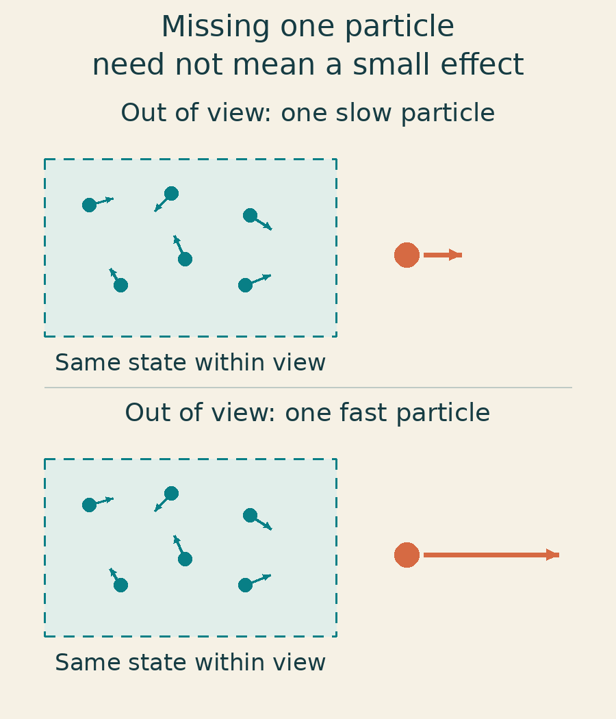
The scheme therefore adds, at both endpoints, a weighted total covering every particle. Each particle’s weight is

$$W(x,v)=1+|x|+|v|^2$$

$x$ is position and $v$ is velocity; $|x|$ is the distance from a reference origin, and $|v|^2$ is proportional to kinetic energy. All terms again use the model’s fixed dimensionless units. Summing $W$ over every particle and normalizing by the known scale simultaneously constrains the particle number and the contributions of distant and fast-moving particles. This scale is determined by the preparation parameters, and its ratio to the mean particle number tends to one in the limit.

Under the paper’s conditions, the absolute values of the logarithmic weights are bounded by a constant multiple of $W$. Subtracting the minimum contributions from the bins within view from the global total therefore gives an upper bound on the weighted contribution outside the field of view. If this bound is small enough, each individual readout comes with a guarantee that the omitted score is small. This approach does not require assuming that potentially troublesome, unusually fast particles are already sufficiently rare in the newly prepared gas.

The conclusion is that, after specifying a positive number smaller than $a$, denoted $\eta$, as the allowed loss in the exponent, one can choose the bins, readout ranges, precision, and acceptance rule before taking the sphere diameter to zero. The acceptance rate for genuinely reversed samples still tends to one. The negative logarithm of the false-positive probability, normalized by the mean particle number, has a limit inferior of at least $a-\eta$ and a limit superior of at most $a$. In other words, even if there is no single limit, its leading exponent is bracketed by two bounds only $\eta$ apart. The loss can be made arbitrarily small by choosing a new finite apparatus with sufficiently fine resolution.

This does not mean that one fixed instrument necessarily achieves the exact full exponent. The fixed precision applies to the normalized collective readouts; it does not fix the total cost of measuring ever more particles. If instrument noise is included, sufficiently accurate, guaranteed error bounds are also needed. Occasional errors without warning could overwhelm the otherwise exponentially rare false-positive events. The paper proves the existence of a readout scheme meeting these conditions; it does not present an experimental apparatus that has been implemented.

The direction of time is also written into the preparation

Linking correlations between particles to entropy is an old idea in statistical physics. This work advances it by connecting correlation information, the likelihood difference between two preparations, and the false-positive exponent of an observable test within a specific hard-sphere model. It makes the statement that “a genuinely reversed gas is special” something that can be calculated and examined in terms of finite-precision readouts.

The scope of these conclusions is equally specific. The gas occupies all of space, and a finite observation interval is chosen in advance. The Boltzmann equation must have a regular solution satisfying the prescribed bounds over that interval, and the initial state must meet positivity, spatial decay, and moment conditions. The paper gives an example of a smooth initial state whose velocity distribution has different widths in different directions, proving that a positive entropy increase does occur over a short but nonzero time interval. It does not prove that arbitrary initial states meet the requirements over arbitrarily long times. The material supplied for this article is a working draft; the results are mathematical derivations, with no experimental or numerical simulation data.

Making the conclusions more practical will require knowing how large the errors are at finite particle numbers, how many bins are needed to retain a given fraction of the exponent, and how to measure the weighted total covering all particles in practice. These questions require new quantitative estimates or measurement schemes.

The opening question now has a clearer answer: copying a gas’s table of single-particle statistics does not copy its past. The collective correlations left by that past allow the genuinely reversed gas to retrace its path. Under the same statistical description, the chance that a newly prepared gas happens to pass the specified test is constrained by an exponent set by the entropy increase. The microscopic rules always permit reversal. This quantitative difference between the directions of time comes from how we prepare the gas; why a low-entropy past is the starting point remains outside the scope of this result.

---

Research source: Entropy, Correlations, and Observable Reversal in a Dilute Hard-Sphere Gas, working draft revised September 5, 2026. The article’s scientific narrative and illustrations are based on this draft; the cover and body illustrations are all original drawings created with code.