
If a receiver knows that only two kinds of signal can arrive, why should its instrument offer a third possible outcome? In the quantum world, an instrument reading does not always identify the signal directly: the receiver must still infer which preparation produced it. For a qubit, the surprising point is this: a simple two-outcome measurement suffices to maximize what we learn, and one also suffices to minimize how often we guess incorrectly. But researchers at Gewu have proved that, for some quantum signals, three outcomes strictly outperform two when both goals matter. The extra outcome preserves evidence that the two scoring rules value differently.

Imagine a transmitter preparing one qubit at a time. It chooses a state labeled “0” or “1” according to probabilities agreed upon in advance—the prior probabilities. The receiver knows what the two states are, but not which was chosen this time. It must identify the label as well as it can from the record left by a single measurement.
If the two states are orthogonal, meaning that quantum theory allows them to be distinguished perfectly, the problem is straightforward. Under ideal conditions, for example, single photons with horizontal and vertical polarization can be directed to two different outputs. But an arbitrary pair of preparations need not have this property. Photons with similar polarization directions may emerge from the same output; if the preparations also involve random mixtures, distinguishing them becomes more complicated.
This difficulty makes the receiver's design consequential. The measurement determines which differences become classical records, and subsequent processing can use only the records already made. Yet a “good record” can mean different things. A receiver may simply want to make an immediate binary choice as reliably as possible, or it may need to preserve the full information about how certain the label is for further processing. The paper investigates how these two requirements change the optimal measurement.
How Often You Guess Correctly, and How Much You Know
Suppose that, after a particular light on the instrument turns on, you judge that the signal has an 80% chance of coming from “0.” This probability, assessed after seeing the outcome, is called a posterior probability. It describes our judgment about the preparation label, a separate matter from the state of the quantum system after measurement.
If you must guess a label immediately, you choose “0,” with a 20% chance of being wrong. Make the same optimal choice for every possible reading, then average over how frequently the readings occur, and you obtain the minimum average error probability for that measurement.
The information calculation asks a different question: how much uncertainty does the reading remove on average? Information theory measures uncertainty using entropy. For a binary choice, entropy is highest when the two possibilities are equally likely and zero when the answer is certain. Subtract the average entropy remaining after the reading from the entropy before it, and you obtain the mutual information between the label and the reading.
Both measures start from the same intuition: greater certainty is better. But they score different degrees of certainty differently.
A purely probabilistic example makes the distinction clear. Suppose the two labels are initially equally likely. Readout scheme A always changes the probabilities to “three-quarters versus one-quarter,” with an equal chance of favoring either label. Guessing the more likely label therefore gives an average error probability of one-quarter.
Scheme B leaves the probabilities at “fifty-fifty” half the time and supplies a strong “99% versus 1%” judgment the other half. Its average error probability is 25.5%, slightly higher than A's, yet its mutual information is about 2.4 times as large. B often offers no help, but at other times makes things very clear. The two scoring rules evaluate this distribution differently.
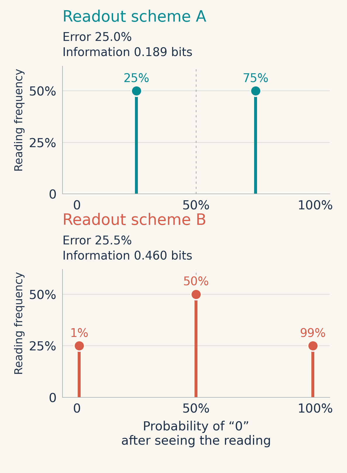
This example proves no advantage for quantum measurements. It shows only that “fewer wrong guesses” does not by itself imply “more knowledge.” Returning to quantum systems, we must answer a more demanding question: which posterior-probability distributions are actually allowed by a given pair of signals?
Both Endpoints Are Simple; the Middle Can Be Different
For a qubit, an ordinary orthogonal measurement selects a pair of mutually orthogonal basis states and gives two possible outcomes. The two outputs of a polarizing beam splitter provide an intuitive example: rotating the measurement basis changes which differences between inputs are more readily revealed at the outputs.
Quantum theory also allows generalized measurements. By letting the signal interact with an auxiliary system and then reading out the enlarged system, we can obtain more than two possible outcomes. Mathematically, each outcome is described by a matrix. Together, these matrices must ensure that, for any input, the outcome probabilities are nonnegative and sum to one. Increasing the number of outcomes also gives us more freedom to design their probabilities.
More freedom, however, is not always useful. For two quantum signals, an orthogonal measurement can always maximize mutual information. Andreas Keil has already proved this for qubits. Research by Árpád Varga, Peter Adam and János A. Bergou has also analyzed information-optimal measurements, showing that they can differ from minimum-error measurements. Keil's paper and the paper by Varga and colleagues discuss these questions, respectively.
The researchers at Gewu went further, building a framework from posterior probabilities that both finds an information-optimal measurement and characterizes which measurements with finitely many outcomes attain the same optimum. The key is to express in matrix form how much a reading increases a label's probability relative to its prior probability, then optimize an information upper bound supplied by these matrices. A binary label has only one independent probability: knowing one determines the other. In the paper's construction, the two optimized matrices are likewise generated by a single matrix, so they can be decomposed along the same set of orthogonal directions. Measuring along those directions actually attains the information upper bound.
This reasoning explains why a complicated generalized measurement can be reduced to an orthogonal measurement when information is the objective. Even if the original two signal states cannot be decomposed along the same set of orthogonal directions, the optimized matrices can still share measurement directions. The paper also provides upper and lower bounds on the optimal information value during computation, making it possible to assess how far a current receiver scheme is from the goal.
The other endpoint also has a simple answer: the Helstrom orthogonal measurement can minimize the error probability. But simplicity at both endpoints does not mean that they select the same basis.
The receiver can therefore make a trade-off between information and error. The paper uses a weighted score:
Here, is the mutual information between the label and the reading, is the minimum average error probability after the reading, and is a nonnegative weight penalizing errors. Once the unit of information is fixed, zero weight means seeking only the most information; as the weight increases, the receiver places ever greater emphasis on reducing errors. The formula compares the information obtained from the reading with the quality of the resulting judgments. It does not measure the disturbance that the measurement causes to the quantum state.
The researchers at Gewu proved that, for two distinct, full-rank qubit states, an optimal generalized measurement with at most three outcomes exists at every weight. The comparison holds the two labels' prior probabilities fixed, with both nonzero. For a qubit, “full rank” here requires a mixed signal state: a probabilistic mixture of different pure states, excluding the boundary case of a single pure state. More strongly, for some such signal pairs, the optimal score with three outcomes is strictly higher than that of any orthogonal measurement throughout an entire interval of weights.
The third outcome does not mean “unable to decide; discard this trial.” All three outcomes are retained, and all enter the information and error statistics. The final judgment is still between two labels. What has been added is a different strength of evidence, not a third kind of signal.
Nor can we match this performance by tossing a coin to switch randomly between orthogonal bases. If the choice of basis is independent of the signal and the record of which basis was used is retained, the overall score is a weighted average of the individual orthogonal measurements' scores. It cannot exceed the best of them. Discarding the basis record cannot improve performance either. The advantage therefore comes from the more general measurement itself.
How Three Outcomes Are Proved Necessary
The original difficulty is that a generalized measurement can have many outcomes, each corresponding to a matrix. Searching these matrices directly makes it hard to know when every possibility has been covered.
Posterior probabilities offer a way to reformulate the problem. A qubit state can be pictured as a point in a ball: the surface represents pure states and the interior mixed states. Mixing pure states with given probabilities amounts to taking a weighted average of their surface points. Mixing the two signal states according to the labels' priors gives a fixed average state.
The researchers at Gewu transform the matrices describing the measurement so that each refined measurement outcome corresponds to an auxiliary pure-state point on the surface of the ball, weighted by the probability of that outcome. The weighted average of all the points must equal the fixed average state exactly. Conversely, such a decomposition can be converted back into a valid measurement. These auxiliary points are tools for reformulating the measurement problem; they do not mean that the instrument actually prepares the input in those states.
In this picture, each point's position determines the corresponding posterior probability and thus its contribution to the weighted score. Using the shape of the scoring function, the researchers at Gewu further proved that, when seeking an optimal scheme, the points can be placed on a semicircular arc in a single plane. The question then becomes: which points on the semicircle should we choose, and with what probabilities, to reproduce the fixed mean while maximizing the average score?
Only three quantities need to be fixed: the sum of the probabilities, which is one, and the mean coordinates in the two directions within the plane. More than three points with positive weights introduce extra freedom to redistribute those weights while leaving all three quantities unchanged. Adjusting them in a direction that does not decrease the score progressively eliminates surplus points. This is the geometric reason that three outcomes suffice.
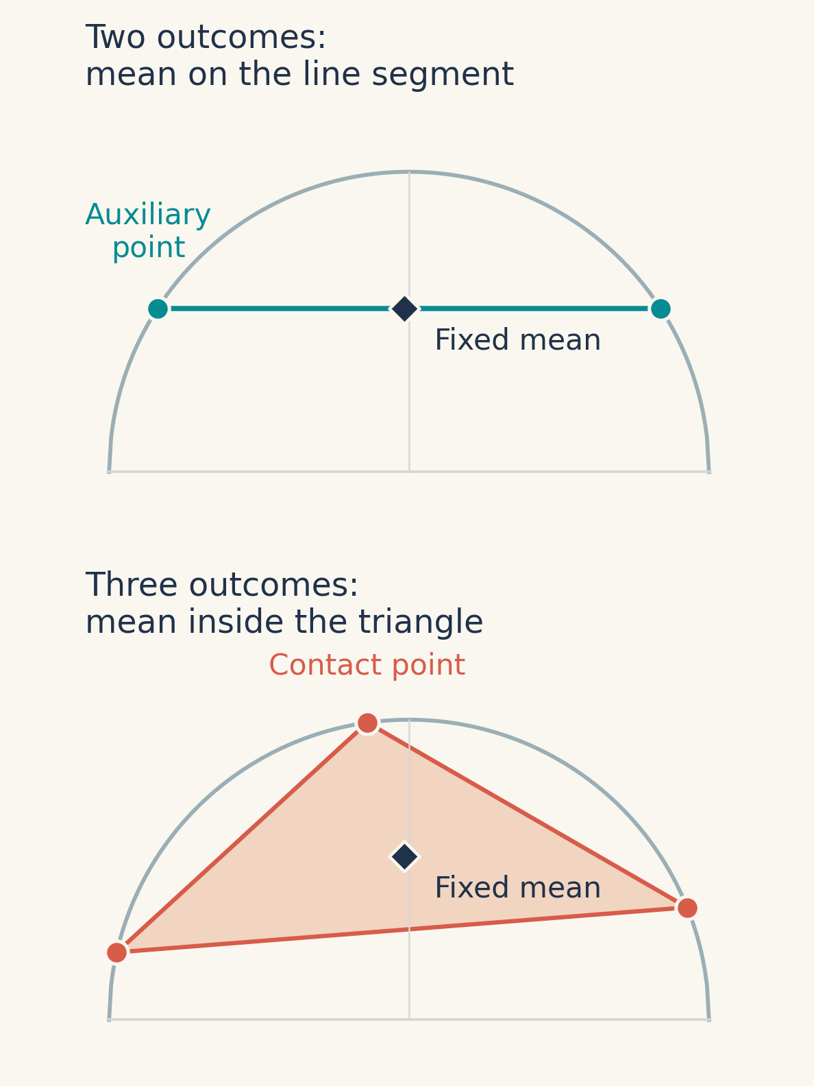
But “sufficient” does not yet mean “necessary.” To establish necessity, the researchers at Gewu constructed an upper bound on the score for all candidate schemes, with equality at exactly three particular points. Reaching the bound requires choosing points from these three. If the fixed mean lies inside their triangle, no two vertices can reproduce it: all three weights must be positive. This rules out every optimal scheme consisting of two auxiliary points. For a qubit, any generalized measurement with only two outcomes can be implemented by first performing an orthogonal measurement and then adding classical randomness to its readings. Adding this randomness can neither increase information nor lower the minimum error probability. Thus, an optimal score beyond the reach of orthogonal measurements is also beyond the reach of any two-outcome scheme.
This strict gap also survives small changes in the weight, so it does not occur only at an isolated parameter value. The paper gives a mathematical existence proof and illustrates examples through numerical scans. It does not, however, prove that every pair of mixed states has this advantage. If the same orthogonal measurement already optimizes both endpoints, no trade-off is required. For general signal pairs, how many separate intervals of weights can favor three outcomes remains an open question.
Who Will Use the Measurement Record?
There is no “best way to read” a pair of signals independent of its purpose. The paper also brings this point into a separate error-correction model: three qubits form a repetition code, with only random bit flips considered. Auxiliary qubits supply check outcomes, and a decoder combines records from multiple rounds to decide which positions need correction. There is no additional ideal check at the end. Under the recovery procedure specified by the model, the recovery risk equals the probability of failing to identify the complete error pattern correctly.
In an example with three rounds of checks and a 2% probability of a flip per bit per round, changing only the basis of the measurement at the final location reduces the local mutual information from approximately 0.04385 bits to 0.04196 bits. The local error probability stays at approximately 10.8621%, yet the final recovery risk falls from approximately 15.9486% to 15.8539%, a relative reduction of about 0.594%. This happens because the decoder also uses the other check records. The two local summary scores do not capture the full role of these records when used together for error correction.
This calculation does not demonstrate the three-outcome advantage in hardware. The modified measurement is itself orthogonal, and the results come from finite enumeration under a particular stochastic noise model. The example shows that even assessing information and error probability together may not suffice to select the readout best suited to the final task.
Bringing the three-outcome theorem to a practical receiver will require comparing auxiliary systems, control errors and readout costs. Extending the mathematical result will require determining how many outcomes higher-dimensional systems need, and how boundary cases such as pure states change the trade-off. These questions call for new implementations or proofs.
The opening question thus has a more precise answer. Having only two labels to distinguish does not require an instrument to leave only two kinds of evidence. To know whether the third outcome is worth keeping, first ask how that evidence will ultimately be used.
Research source: Posterior Algebra of Binary Quantum Measurements: From Shor’s Orthogonal-Measurement Conjecture to Information–Error Pareto Frontiers. Both the core theorems and the error-correction example in this article are based on this paper. The three-outcome results appear in the main text and Appendices G–L; the error-correction example appears in Appendices M–O. The illustrations are original programmatically generated artwork for this article. Figure 1 is a teaching example; the cover and Figure 2 are conceptual illustrations.