The precision limit of quantum currents lies at a filter’s edges

A tiny wire does not always deliver the same number of electrons over equal intervals of time. Stabilizing the flow usually means increasing the cost of driving the electrons forward; quantum coherence, however, can break through a precision limit that applies to a class of classical systems. Researchers at Gewu have taken the question further: how far can making a device longer extend this advantage? They find that the answer depends on how well the device selects particles by energy. The closer it comes to “letting everything through inside a window and blocking everything outside,” the steadier the current. A finite chain, however, always leaves noise at the window’s edges.

Looking beyond the average current

Imagine a tiny device delivering electrons continuously. The average number it sends out per second tells us only how fast it operates. If its output varies from one interval to the next, it will struggle to provide a steady flow. If particle-passage events are used to keep time, fluctuations in the count also become errors in the time reading.

Studying this reliability requires repeated records of the net number of particles passing through over a long observation period. As the observation time increases, both the mean count and the variance of the count—a measure of how widely the results are spread—grow approximately in proportion to time. Dividing each by the observation time gives the mean particle flow rate $j$ and the variance growth rate $d$. At the same mean flow rate, a smaller $d$ means steadier output.

There is another quantity to account for: entropy production. It measures the thermodynamic cost of irreversible operation in the device and its environment, such as the increase in entropy accompanying energy dissipation. Taking Boltzmann’s constant as the unit of entropy and writing the total entropy production per unit time as $\sigma$, we can form a dimensionless measure:

$$\mathcal{P}=\frac{\sigma d}{j^2}.$$

This is also the product of “entropy produced per net particle transferred” and “the ratio of the variance growth rate to the mean flow rate.” The smaller this uncertainty product, the better the device’s combined performance in dissipation and counting noise. Simply speeding up all processes together changes the flow rate, the variance growth rate, and the entropy production rate at the same time; it does not automatically reduce the product.

For an important class of classical models, this product is at least $2$. These models describe a system through random jumps: the jump rates do not change with time, the next jump depends only on the current state, and the rates of forward and reverse transitions satisfy the relevant thermodynamic conditions. Such a process is called a Markov jump process. Its “thermodynamic uncertainty relation” means that making the output steadier carries a corresponding cost in entropy production. This classical constraint has specific conditions of applicability; it is not a claim about all stochastic processes.

Quantum systems have an additional way to organize motion. Before reaching the exit, a particle can be in a superposition of different positions; the quantum amplitudes for different propagation processes retain their phase relationships and can interfere with one another. This coherence gives currents a chance to break through the classical lower bound above. In 2021, drawing on studies of small open quantum systems, Paul Menczel, Eetu Loisa, Kay Brandner, and Christian Flindt conjectured that the uncertainty product could approach zero arbitrarily closely as the available degrees of freedom increased. Their original paper brought the relationship between device size and precision into focus.

Researchers at Gewu have now provided an answer for a specific system: a chain of noninteracting fermionic modes. A mode can be thought of as a quantum site along the chain that a particle can occupy; fermionic statistics allow at most one particle in each mode. Electrons are fermions, and an array of quantum dots offers one physical picture of this kind of model. In the model, particles can move coherently between neighboring modes, while the two ends exchange particles with the environment. The environment’s influence is described by memoryless injection and removal processes, and interactions between particles within the chain are neglected.

The results of this work are mathematical proofs and design constructions, not yet an experimental device that reaches the limit. The question they answer is: within this model, how much improvement is possible, even when every connection is carefully tuned?

Randomness lingers where the door is half open

To understand the chain, it helps to start with particle energy. For an incoming particle with energy $E$, the chain has a transmission probability $T(E)$: the particle may pass from entrance to exit, or it may be reflected back. Adjusting the coupling strengths between modes changes the transmission probabilities at different energies, turning the whole chain into an energy filter.

The ideal shape is a window with perfectly sharp edges: complete transmission inside, complete reflection outside. What is being selected here is particle energy, not unwanted data removed from the records after the fact.

Why does this reduce noise? If particles of a given energy are reflected every time, they make no random contribution to the transmission count. If they pass through every time, the chain no longer introduces the random partitioning of “through this time, blocked the next.” The regions most prone to this noise are those with transmission probabilities between the two extremes, like a half-open door. Their noise contribution contains the factor $T(E)[1-T(E)]$, which is zero at complete transmission or complete reflection and reaches its maximum when the transmission probability is one-half. This component is called partition noise.

Fermionic statistics are also crucial. When the incoming states within the window are sufficiently occupied and the exit side is sufficiently empty, the occupancy limit on each mode works together with nearly deterministic transmission to suppress counting fluctuations. Perfect transmission alone does not eliminate every source of noise; reverse transport induced by the environment still has to be addressed separately.

Adding up the partition noise over all energies and dividing by the total transmission weight gives

$$F_0=\frac{\int T(E)[1-T(E)]\,\mathrm{d}E}{\int T(E)\,\mathrm{d}E}.$$

The integrals cover the entire energy axis. This $F_0$ is the Fano factor in the limit of sufficiently strong unidirectional driving—that is, $d/j$ in that limit. It compares relative counting noise in transport, rather than the total absolute noise. An ideal rectangular window would make the numerator zero.

The difficulty lies precisely at the window’s edges. Can a finite number of connections and modes make the transmission fall from nearly one to nearly zero over an extremely narrow energy range? Kay Brandner and Keiji Saito previously studied a class of quantum-dot chains whose transmission curves approach a rectangle as the chains grow longer, with partition noise falling roughly in inverse proportion to the number of modes. This study of coherent transport demonstrated the potential of energy filtering. But what one design can achieve does not establish the limit for all designs.

Researchers at Gewu found a unified description: for a nearest-neighbor chain with $n$ modes, the transmission can always be written as

$$T(E)=\frac{1}{1+Q(E)}.$$

Here, $Q(E)$ is a polynomial of degree $2n$ that is nonnegative at real energies. The degree is the highest power of energy appearing in the polynomial. Where $Q$ is very small, transmission is almost complete; where $Q$ is very large, reflection is almost complete. This form follows from the chain’s geometry: there are no branching routes between its ends, and the numerator in the expression for propagation from one end to the other is the product of all the neighboring coupling strengths, independent of energy. Combined with the fact that transmission and reflection probabilities sum to one, this constrains the complex transmission profile to the form above.

A quantum transport problem thus becomes a problem about the shape of a polynomial.

How chain length shapes the window’s edges

Polynomials can bend and oscillate, but at finite degree they cannot stay within a prescribed range over an interval of nonzero width and then rise arbitrarily steeply at its edges. A polynomial inequality established by the mathematician Andrey Markov bounds the maximum slope on a scale proportional to the square of the degree. This theorem about polynomial slopes is separate from the Markov models of random jumps discussed earlier.

Applying the inequality to a transmission window shows why noise cannot be eliminated completely. Within a window, $Q$ remains small, but it must rise at the edges. Because its slope is finite, there is always a region near an edge where transmission is neither close to zero nor close to one. This region necessarily contributes partition noise. Increasing the number of modes can narrow it, but cannot do so arbitrarily fast. Even if the transmission spectrum is split into multiple windows, the same constraint appears at the edges of each window.

Adding up the contributions from these regions, the researchers at Gewu proved that $F_0$ cannot fall below $1/(18n^2)$ for any chain satisfying the model. This lower bound allows different mode energies, different coupling strengths between neighbors, and unequal contact strengths on the left and right; it does not apply only to a particular symmetric chain.

A lower bound, however, tells us only that no design can do better than this. To determine whether inverse-square scaling really is the key, one must also construct designs that approach it.

The answer comes from a family of functions already used in the mathematics of filters: normalized Gegenbauer polynomials. Transmission spectra designed with them have only small ripples inside the window, fall rapidly near the edges, and have sufficiently small tails outside. The steepness of the edges is not the only consideration: ripples inside the window and tails outside it also produce noise. Accounting for all these contributions, the researchers at Gewu proved that $F_0$ for this class of transmission spectra is less than $6/n^2$.

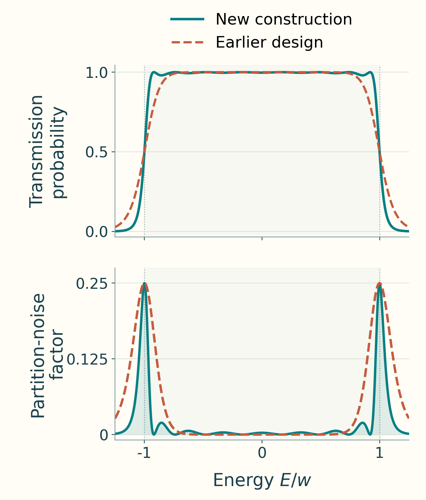
A crucial step follows: proving that this elegant curve actually corresponds to a physically allowed chain. Working backward from the target transmission spectrum to the coupling strengths between modes, the researchers at Gewu proved that a corresponding chain exists at every finite length, with positive, left–right symmetric coupling strengths and equal contacts at its two ends. Only then do the lower bound—“no design can improve faster”—and the upper bound—“a design achieving this rate exists”—meet in their scaling with chain length.

But $F_0$ is not yet the final uncertainty product. The environment can send particles forward, but it can also make them jump backward. Making transport sufficiently biased in one direction requires stronger driving.

The paper uses a dimensionless parameter $A$ to describe the bias between forward and reverse transitions at each contact: the ratio of the forward to reverse rates is $e^A$, where $e$ is the base of the natural logarithm. The larger $A$ is, the rarer reverse transitions become. But a particle completing a net transfer must undergo exchanges at both ends, producing $2A$ of entropy in this model. Suppressing thermal noise therefore also increases the weight of partition noise in the dissipation–precision product.

Both requirements must be met together. Choosing $A=2\ln n$, so that the driving grows with the natural logarithm of the number of modes, brings the contributions of thermal noise and residual partition noise to the product down to the same order. The researchers at Gewu ultimately proved that, for chains with at least three modes,

$$\frac{\ln n}{18n^2}\leq\mathcal{P}_{\min}(n) <33\frac{\ln n}{n^2}.$$

$\mathcal{P}_{\min}(n)$ denotes the smallest product that can be approached, for a given number of modes, among the allowed chain designs and finite driving strengths. The constants on the two sides differ, so the study does not determine the exact optimal value. It determines the rate of decrease: an inverse square multiplied by a slowly growing logarithm. Compared with the roughly $\ln n/n$ improvement of the earlier class of chains, this shows that careful design can gain an additional factor of chain length.

Nor is this improvement achieved by bringing the particle flow to a halt. For the construction that attains this scaling, the current approaches a nonzero value as long as the energy-window width is held fixed. Entropy production per particle, however, grows as $4\ln n$. The product shrinks because relative noise falls faster; this cannot be interpreted as the dissipation per transferred particle also approaching zero.

Who maintains the flow through a more precise window?

Maintaining a current at fixed window width might sound as though the full cost has already been accounted for. But the chain has two easily overlooked components: the contacts through which it exchanges particles with the environment.

Coupling an endpoint to the environment gives its energy level a certain linewidth. This linewidth reflects how the contact broadens and damps the mode and serves as a coupling scale in the model; it is not the number of particle jumps actually recorded. The weaker contact can limit the entire chain, and increasing the coupling at the other end cannot compensate without limit.

The researchers at Gewu proved that the smaller of the two contact linewidths sets a budget for the entire transmission spectrum. The closer transmission is to perfect, the more of this budget is consumed per unit energy width: reducing the reflection probability by the same factor again requires another fixed amount of budget. To sustain extremely low reflection over a window of nonzero width, the contacts must therefore grow stronger as the precision requirement increases. This relation follows the logarithmic approach Robert Fano used in studying broadband circuit matching, linking filter design to resource limits in quantum transport.

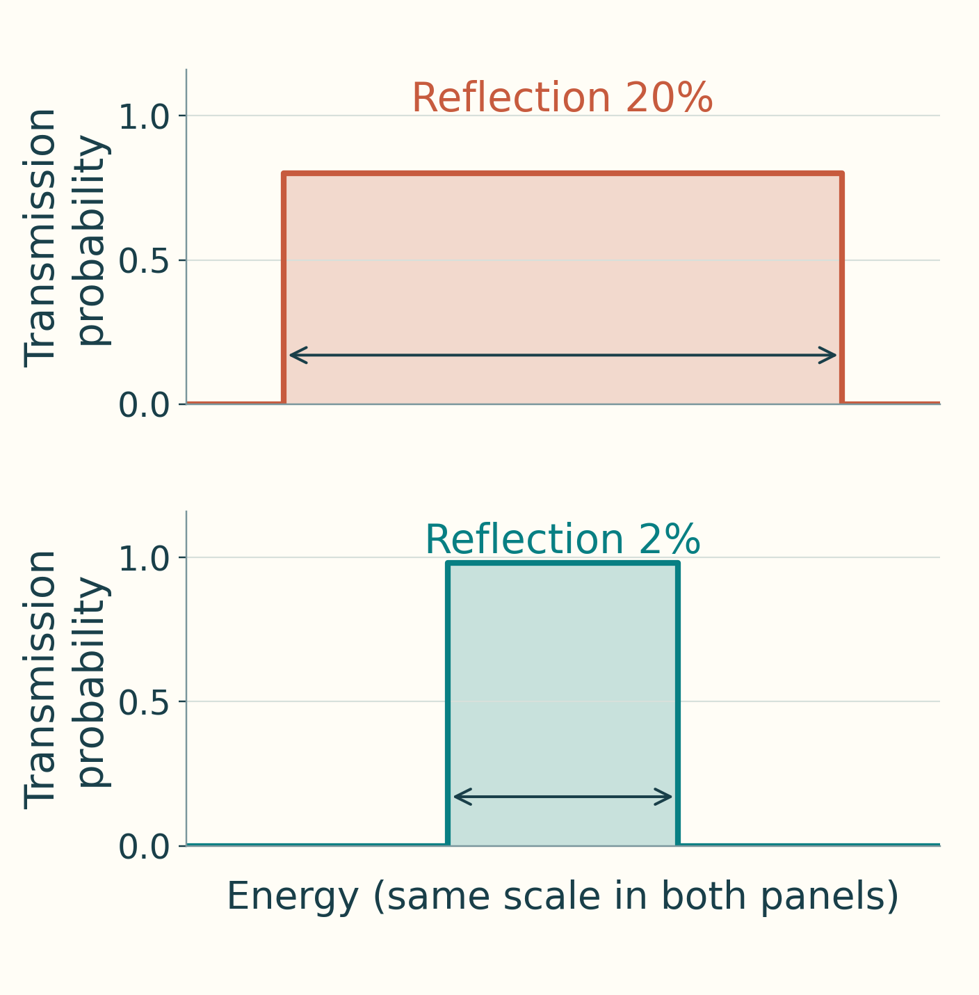
This budget has a direct consequence: if contact linewidths remain bounded while the uncertainty product is to approach zero, the current must approach zero too. The device can still be extremely precise, but it cannot improve without limit at a finite flow rate. The paper also constructs chains in which all neighboring coupling strengths are bounded, proving that this “ever more precise, ever slower” limit is indeed attainable.

Conversely, maintaining the same current requires the contact cost to grow. The paper establishes the most economical growth law for the contacts: as the target product becomes smaller, the ratio of the weaker contact’s linewidth to the current grows primarily as the logarithm of the reciprocal target product, with a still slower double-logarithmic correction. Another class of chains, designed using Chebyshev polynomials, can attain this law. Here the quantity being optimized is the contact resource; earlier it was chain length. Whether a single device can attain both optimal scalings remains an open question.

These results also define the boundaries of the conclusions. In a fermion chain where each mode has only two states, empty and occupied, $n$ modes correspond to a quantum state space of dimension $2^n$. Using these chains and auxiliary energy levels, the paper proves that, within the broader class of thermal-transition models it specifies, there is no positive lower bound independent of dimension, thereby realizing the behavior of approaching zero envisaged in the 2021 conjecture. But the optimal rate of decrease in that broader class remains unknown; the chain’s inverse-square law cannot be extended directly to all quantum devices.

One concrete next question is whether, in quantum-dot arrays satisfying the assumptions about coherent transport and the contacts, relative noise under sufficiently strong unidirectional driving can approach inverse-square scaling. Interactions, loss of phase coherence, and errors in tuning coupling strengths in real devices all require separate study. This theory provides a yardstick for comparing experimental designs: first ask whether the edges of the particle-energy window are steep enough, then ask what sustains the window’s width and the flow. Quantum coherence opens up possibilities beyond classical limits, while finite chain length and finite contacts determine how far those possibilities extend.

---

Research basis: The supplied paper and supplementary material, The Minimal Uncertainty Product of Noninteracting Fermion Chains Scales as log n/n² in the Number of Modes, manuscript dated October 21, 2026. All new results described in the text come from this manuscript; the historical-background links lead to the corresponding original studies. The cover and figures were created programmatically as original illustrations for this article.