An extra channel leaves a molecular machine’s fluctuations unchanged

To understand the internal structure of a molecular machine, we may not be able to see every step it takes, but we may be able to measure the random fluctuations as it works. Physicists already know that these fluctuations are jointly constrained by energy dissipation and internal cycles. Researchers at Gewu have now found that, in a class of idealized networks, adding a new channel that the machine actually uses can leave entropy-flow fluctuations entirely unchanged. What changes instead is the theoretical minimum fluctuation level. This distinction determines what we can learn when inferring structure from noise—and what we might miss.

An enzyme may first bind its substrate, then change shape, release a product, and finally return to its starting point. This process can repeat continually, but individual cycles do not run on a fixed schedule: sometimes the wait is longer, and sometimes the machine even steps backward. When many machines work at once, these differences tend to average out; when we observe a single small system, they become noise that cannot be ignored.

Noise can also offer clues. If different internal structures permit different minimum noise levels, a measurement may rule out some structures. Without first identifying every intermediate state, researchers can ask: what processes must a machine contain, at a minimum, to produce such a steady output? This is what makes thermodynamic lower bounds on fluctuations interesting.

Ruling out one structure, however, is different from identifying a unique structure. The new paper provides an exactly calculable example: two different channel structures can produce identical long-time entropy-flow statistics. To understand this result, we first need to see precisely what the theory constrains.

Keeping an entropy ledger for every jump

Draw the machine’s internal states as points and its allowed state changes as connecting lines, and you have a network. These lines have no physical length in space; they simply indicate that two states can interconvert directly. Each line permits transitions in both directions, whose rates may differ.

A rate does not mean “a fixed number of jumps every second.” It describes the probability of a jump occurring within a very short time. For example, a rate of 2 per second means that, over a sufficiently short interval, the jump probability is approximately 2 times the duration of that interval in seconds. Even at a fixed rate, the actual waiting time for each jump remains random.

The model studied in the paper also requires that the probabilities for the system’s next step depend only on its current state, not on its earlier history. This is a Markov model. After enough time, the probability of occupying each state no longer changes, and the system is in a steady state. A steady state does not mean that motion has stopped: the average forward and reverse flows can differ, and the machine can continue working and dissipating energy.

To connect jumps with thermodynamics, we can enter an entropy contribution for each step in a ledger. In the thermodynamic description of these models, a jump from state $i$ to state $j$ corresponds to a dimensionless increase in environmental entropy of $\ln(k_{ij}/k_{ji})$. Here, $k_{ij}$ and $k_{ji}$ are the rates in the two directions, and $\ln$ denotes the natural logarithm; entropy is measured in units of Boltzmann’s constant. If the two rates are equal, the entry is zero. If the forward rate is twice the reverse rate, a forward jump contributes $\ln 2$ and a reverse jump $-\ln 2$.

The sum of all entries during an observation time $t$ is denoted by $S(t)$. This is the cumulative entropy flow into the environment. Along a random trajectory, the total can temporarily decrease, but in a nonequilibrium steady state, its long-time average growth rate is positive and equals the entropy production rate. Here we want to compare not only the average growth, but also how much this total fluctuates across repeated observations.

The paper measures these fluctuations using a quantity called the Fano factor:

$$F_s=\lim_{t\to\infty}\frac{\operatorname{Var}[S(t)]}{\langle S(t)\rangle}.$$

The angle brackets denote an average over many observations. $\operatorname{Var}$ denotes the variance: the average squared deviation from the mean. The subscript $s$ indicates that the observed quantity is entropy flow. Here, at sufficiently long times, both the mean and the variance grow approximately in proportion to time, and their ratio approaches a constant. With the same entropy units and definitions, a larger Fano factor means larger fluctuations per unit of mean entropy flow.

Why pay attention to the entropy ledger? It brings the thermodynamic cost of sustaining directed motion and the associated random fluctuations into a single description. In 2015, Andre C. Barato and Udo Seifert proposed the thermodynamic uncertainty relation: in the steady-state models to which it applies, greater output precision requires a greater cost in dissipation. For the entropy flow considered here, it gives a simple long-time lower bound: $F_s\geq 2$. The original study subsequently inspired work that uses information about the internal network to tighten the bound further.

This “2” is not the noise level a machine should produce, but a boundary it cannot cross. The actual value can be much higher. To raise the boundary further, we need to know which cycles the network allows.

How much driving is there per step around a cycle?

A path that goes around the network and returns to its starting point without revisiting any state along the way is called a simple cycle. Adding the entropy entries for every step gives the total driving around that cycle, known technically as the cycle affinity. It compares the product of the rates around the cycle in one direction with the product in the reverse direction. If the two products are equal, the total driving is zero.

Distributing the same total driving over more steps reduces the average driving per step. The stronger lower bound on fluctuations depends on a parameter $r$: consider every simple cycle with nonzero total driving, divide the absolute value of its total driving by its number of steps, and take the smallest ratio. Taking the absolute value makes the result independent of which direction we call forward.

In 2016, Patrick Pietzonka, Barato, and Seifert proved a fluctuation bound incorporating this parameter. For entropy flow, it requires:

$$F_s\geq r\,\coth\!\left(\frac r2\right).$$

Here, $\coth x=(e^x+e^{-x})/(e^x-e^{-x})$ is called the hyperbolic cotangent. There is no need to memorize this function; what matters is how the boundary changes: the larger $r$ is, the higher the lower bound, and as $r$ approaches zero, the lower bound approaches 2. Information about internal cycles can thus impose a stricter limit than the basic thermodynamic constraint. The 2016 proof also shows that a uniform single-cycle network can attain the corresponding bound.

The new paper first clarifies a detail in applying this result: cycles with zero total driving must be excluded when taking the minimum. Including zero immediately gives $r=0$, losing the improvement. Going along an edge and straight back along the same edge also does not count as a simple cycle here; otherwise, every bidirectional network would contain a cycle with zero total driving. Using a counterexample, the Gewu researchers also verified that substituting the largest driving per step for the smallest gives an incorrect “lower bound” that actual fluctuations can violate.

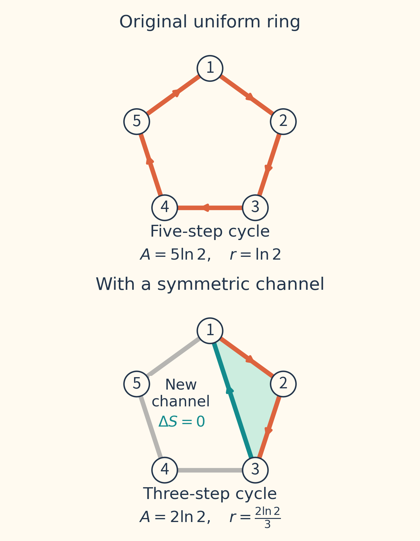
Now consider a five-state ring: every state has a forward channel and a reverse channel, with uniform forward rates of 2 per second and uniform reverse rates of 1 per second. Completing five forward steps gives a total entropy entry of $5\ln 2$, so $r=\ln 2$.

This uniform ring attains the lower bound exactly. Its entropy-flow Fano factor is $3\ln 2$, approximately 2.0794. In this model, the theoretical boundary coincides with the actual fluctuations, making it a useful starting point for comparison.

Adding a channel changes the boundary

The Gewu researchers added a new channel between states 1 and 3. Its rate in both directions is $\varepsilon$; the Greek letter $\varepsilon$ here denotes the transition rate along the added channel. It can be large, or so small that the machine rarely uses this route.

As long as $\varepsilon>0$, a new triangular cycle exists: go from 1 to 2 and then to 3 along the original ring, then return to 1 through the new channel. The first two steps each contribute $\ln 2$. The last step has equal forward and reverse rates and contributes zero. The total driving around this cycle is $2\ln 2$, spread over three steps, giving an average of $2\ln 2/3$ per step.

The five-state network also gains another, four-step cycle, with an average driving per step of $3\ln 2/4$. Comparing these with the original five-step cycle, the three-step cycle gives the minimum. The new parameter is therefore $r=2\ln 2/3$, with a corresponding lower bound of approximately 2.0355, below the original value.

The surprise lies in the actual fluctuations: the Fano factor remains 2.0794. The new channel makes the machine’s entropy flow neither steadier nor noisier.

Simply saying that “the new channel produces no entropy” does not fully explain this result. A route that adds nothing to the entropy ledger could still take the machine to a state where it moves faster or slower, changing the subsequent statistics. The key to the invariance in this example is the uniformity of the original ring.

At any state, the rate of forward jumps along the original ring is always 2 per second, and the rate of reverse jumps is always 1 per second. After the machine uses the new channel, these two rates remain the same as before. Although the machine has reached a different state, the rhythm of its entropy flow has not changed: the opportunities for positive entries and for negative entries are unchanged, while the extra jumps add only zero entries.

The paper turns this observation into an analytical proof. To calculate the full entropy-flow statistics, jumps in each direction are reweighted according to their entropy contributions. On a uniform ring, the total rate of change after reweighting is the same regardless of the starting state. The added symmetric channel contributes both an incoming term and an outgoing term, which cancel in this sum. The quantity governing the long-time entropy-flow statistics therefore retains its original value.

This is stronger than “the mean and variance happen to be the same”: it guarantees that the full set of long-time entropy-flow fluctuation statistics remains unchanged, including rare departures from the mean. This is a mathematical result for the particular networks described above. It does not mean that every trajectory of the machine is identical, or that separately counting jumps along each channel would reveal no difference.

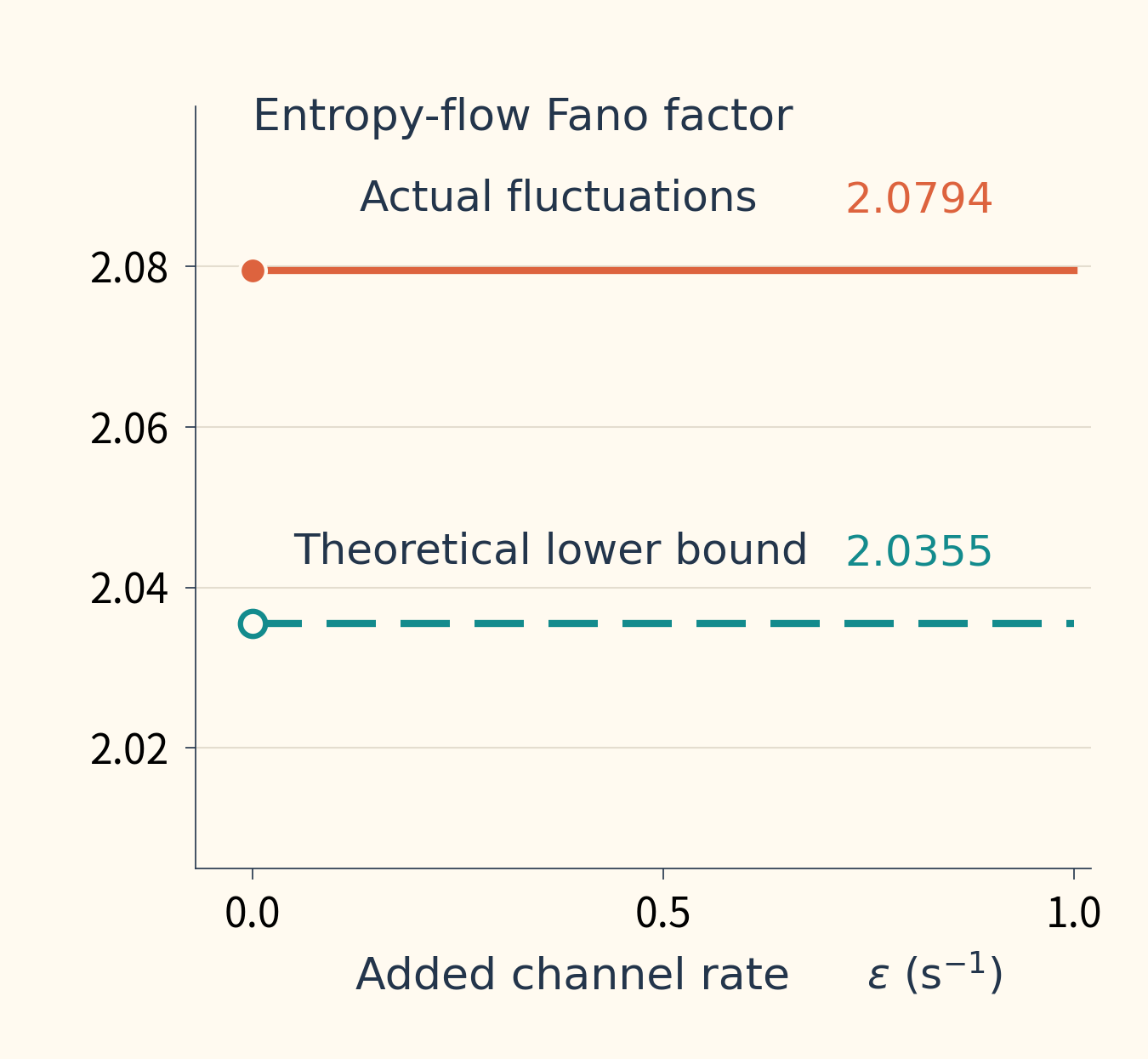
Gradually reducing $\varepsilon$ does not gradually bring the two curves together. Their separation is the same for every positive $\varepsilon$; only when the channel disappears completely does the lower bound return to the actual value. This does not mean that the machine’s physical behavior changes abruptly. Rather, the parameter in the bound asks only whether the route is accessible. It does not account for how often the route is used.

How much structural information does noise retain?

The analytical example explains the mechanism, while computational checks help test the definitions and their implementation. The Gewu researchers enumerated all cases in which the rates on connections in four-state multicyclic networks take values of 1, 2, or 3. This includes the fully connected network and the six labeled networks obtained by deleting one connection, for a total of 877,626 nonequilibrium systems. The study also checked nearly 4.92 million edge currents.

None of these cases violated the fluctuation bounds under examination. But “exhaustive verification” has a specific scope: it refers to a finite rate grid and a specified network size, not every possible machine. Comparisons involving the full fluctuation statistics were also carried out only at a finite number of parameter points. The scan used ordinary floating-point arithmetic, with exact arithmetic for key questions such as identifying zero driving; the reported extreme cases were then rechecked at 80-digit precision and through different computational routes. This is therefore a large-scale computational audit. The validity of the bounds for general models still rests on the earlier mathematical proofs.

Nor does this audit turn the statement “only uniform rings can attain the entropy-flow lower bound” into a general theorem. Within the scope of the paper’s exhaustive search, the networks attaining the bound were uniform single-cycle networks. Whether equality is possible in other cases still requires proof. The symmetric-channel example answers a more specific question: progressively weakening the new channel along this family of networks cannot bring a multicyclic network gradually closer to the lower bound.

For anyone trying to infer structure from noise, this distinction has practical consequences. If a theoretical lower bound lies above the measured Fano factor, it can rule out the corresponding candidate structure, provided the model assumptions apply. But a candidate structure’s lower bound lying below the measured value does not establish that it is the correct structure. Nor can a large gap above the lower bound be directly attributed to poor machine performance: it may also reflect the coarseness of the structural information used in the bound.

There is an even more direct limitation. The original ring and the ring with a symmetric channel have identical long-time entropy-flow statistics. Those statistics alone cannot reveal whether the new channel exists. Distinguishing the two requires additional observations, such as directly identifying jumps between states or counting uses of the new channel. The paper does not prove that all measurable signals are identical.

What other changes to a network can preserve entropy-flow statistics? Which internal structures can be distinguished using different current statistics? These questions left by the paper call for further classification and proof. They concern not whether measuring instruments are precise enough, but how much structural information the chosen observable actually retains.

Return to that rarely used new channel: it truly changes the routes the machine can take, yet leaves the long-time fluctuations of its entropy ledger unchanged. Noise can indeed constrain internal structure, but interpreting that clue requires distinguishing the actual random fluctuations from the theoretical minimum.

---

Research basis: the original paper in the current directory, particularly Sections 4.1, 4.3, 4.4, and 7. The cover and article figures are original illustrations generated programmatically for this feature. The layouts and numerical values of the article figures can be regenerated from the accompanying drawing source files.