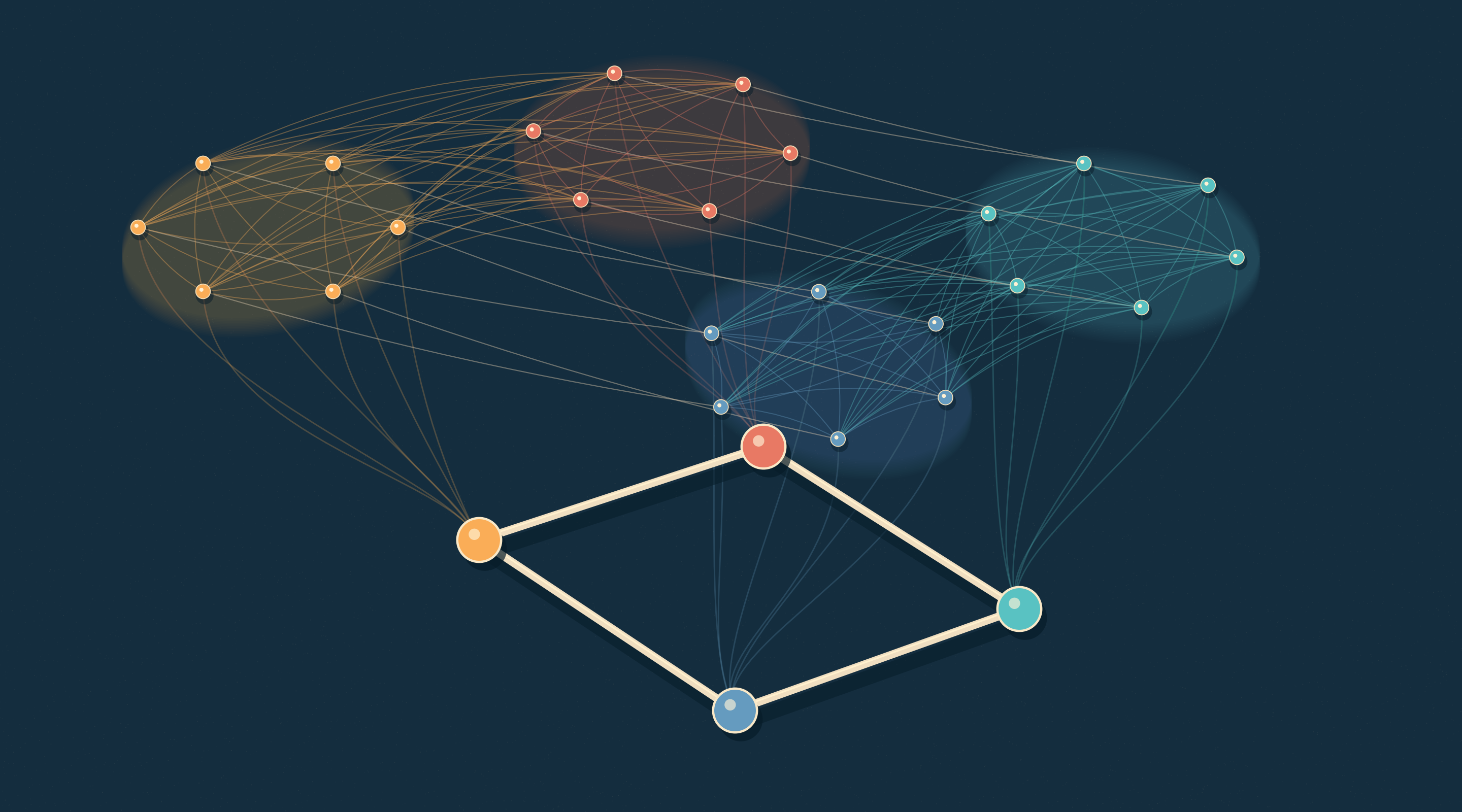
The hidden graph skeleton is simple, but finding it is hard

Four dense clusters of colored edges correspond via thin lines to a clearly defined four-sided skeleton below — Cover: The dense edges above and the four-cycle below symbolize the simple structure revealed by grouping and contracting vertices. The thin lines between the two levels indicate the correspondence between groups and vertices; the image is not the result of an algorithm run, nor does it suggest that the skeleton is unique.

A graph crisscrossed by a dense tangle of edges may hide a simple skeleton: combine certain vertices into groups, and a jumble of relationships can fall into order. But if no one tells you how to group them, does simplicity beneath the surface make the search simple too? The Gewu researcher has proved that even when the skeleton must contain no triangles and be only a little more complex than a tree, deciding whether it exists still encounters a major barrier in computational complexity. The difficulty can lie in choosing the groups, rather than in the skeleton they reveal.

To see this distinction, start with a graph of acquaintances. Each person is a vertex; two people who know each other are joined by a line, called an “edge” in mathematics. If a group of people all know one another, we can collapse them into a single vertex. In graph theory, a set in which every pair of vertices is joined by an edge is called a “clique.” A single vertex can also form a group.

Partition everyone into groups of this kind, with each person belonging to exactly one group. Whenever there was at least one edge between two groups, join the two vertices produced by contracting them. The resulting graph records the connections between groups. A connection between two groups does not mean that everyone in one knows everyone in the other: a single edge between the groups is enough.

The paper interprets this grouping as a “thick model”: the original graph can be viewed as the result of expanding each vertex of a hidden graph into a clique. The hidden graph is called the “thin graph”—what we are calling the skeleton here. “Hidden” means only that the grouping is not supplied to the algorithm along with the input; it does not mean that the original graph actually underwent some expansion process.

Strictly speaking, the model also allows the skeleton to contain extra edges with no corresponding edge in the original graph. For this study, however, all these extra edges can be deleted: deleting edges creates no triangles and cannot increase treewidth, a concept we will come to shortly. It is therefore enough to consider the skeleton drawn from the actual connections between groups, as described above, to answer the original question. This step ensures that we have not quietly replaced the model with a stronger requirement.

The two rows of vertices at the top each form a clique and are joined by four matching edges; contracting the four shaded groups produces the four-cycle below — Figure 1: An example of the base graph in the paper's construction. Every pair of the four vertices in the upper row is adjacent, as is every pair in the lower row; the only edges between rows match corresponding vertices. Orange and blue distinguish the two grouping choices. Corresponding vertices in the two rows make the same choice, producing a four-cycle after contraction. This is not yet the full reduction graph: with this base alone, contracting each entire row to a single vertex is also valid. Drawn from Sections 3–4 of the paper.

Finding a skeleton is appealing because it may let us break a tangled computation into parts. If the skeleton is a tree, it has no cycles that return to their starting point. Working along the tree from its ends, one region at a time, each region needs to exchange information with the rest through only a few interfaces, without recomputing the entire network at every step.

For example, choosing a set of people who do not know one another corresponds to choosing vertices with no edges between them. At most one person can be chosen from any clique. If the cliques are connected in a tree structure, we can record, group by group, which choices of a person are compatible with the choices in neighboring groups, then combine the results from the branches. The benefit of simple structure is concrete here: it limits how many interdependent choices the different parts must consider at once.

A natural question follows: if these groups are not marked, can we find them first? Martin Dyer and Haiko Müller have given a polynomial-time algorithm to decide whether a graph can be contracted in this way into a forest—a collection of disjoint trees. They then asked whether the permitted skeletons could be made slightly more general. Thick Forests

One tool for measuring this generalization is “treewidth.” It measures not how many edges a graph has, but whether the graph can be fitted into small “bags,” linked in a chain or a tree, each containing only a few vertices.

There are two key requirements. Both endpoints of every edge in the original graph must appear together in at least one bag. If a vertex appears in several bags, those bags must form a connected part of the tree of bags. This ensures that no relationship represented by an edge is missed, and that information about the same vertex stays connected throughout the computation. Take the number of vertices in the largest bag and subtract one, then minimize this quantity over all valid arrangements: the result is the treewidth.

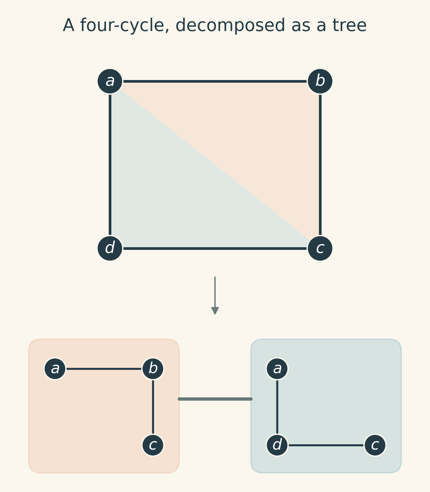
The graphs of treewidth at most one are precisely the forests. With treewidth at most two, each bag needs to contain at most three vertices, and cycles are allowed. A four-cycle, for instance, can be decomposed into two bags of three vertices: one holds the first three vertices, the other the first, third, and fourth, and the two bags are joined. Bags indicate only which vertices need to be considered together; they do not require those vertices to be pairwise adjacent.

A four-cycle is covered by two triangular colored regions; below it, two connected bags hold the first three vertices and the first, third, and fourth vertices, respectively — Figure 2: A tree decomposition of a four-cycle. The orange region above corresponds to the bag containing $a,b,c$ , and the blue region to the bag containing $a,c,d$ ; the colored regions are not additional edges. The two bags below are joined. Every original edge lies within a bag, and the bags containing any given vertex are connected. The largest bag contains three vertices, so this decomposition has width two. The treewidth of this four-cycle is exactly two.

Allowing such skeletons still seems fairly restrictive. But graphs of treewidth two can already contain triangles, and triangles bring known difficulties in recognition. Dyer and Müller therefore narrowed the question further: if the skeleton has no triangles and treewidth at most two, is there still a polynomial-time recognition algorithm? They left this case as an open problem. Thick Forests, Section 7.2

The Gewu researcher's answer is that this recognition problem is NP-complete. In plain terms, if someone supplies a “yes, it exists” answer along with a grouping and a proof of the required structure, we can verify it in polynomial time. But deciding the answer for an arbitrary input graph is at least as hard as an entire class of famously difficult problems. “Polynomial time” means that the running time is bounded by some fixed power of the input size, a standard dividing line for algorithmic efficiency in complexity theory.

This conclusion does not prove that no fast algorithm can exist. It means that, unless the two complexity classes P and NP are equal, there is no polynomial-time algorithm that works for all inputs. Here, P consists of decision problems solvable in polynomial time, while NP consists of problems whose “yes” answers have certificates that can be verified in polynomial time.

To establish this difficulty, the Gewu researcher did not try to enumerate all graphs. Instead, the researcher encoded another known NP-complete problem entirely in the choices of how to group the vertices.

That problem can be explained with a box of beads. Color each bead orange or blue, and supply a list in which each entry specifies three distinct beads. No triple on the list is allowed to have all three beads the same color. For any one triple, this is easy to satisfy. The difficulty is that a bead may recur in many triples, so one color choice affects many conditions at once.

The next step is to turn the beads and the list into a graph, so that “a valid coloring exists” corresponds exactly to “a skeleton meeting the requirements can be found.” Translating one problem into another while preserving its yes-or-no answer is called a “reduction.” The translation must also be efficient enough: it cannot construct an enormous graph and spend all the time needed to solve the problem in advance.

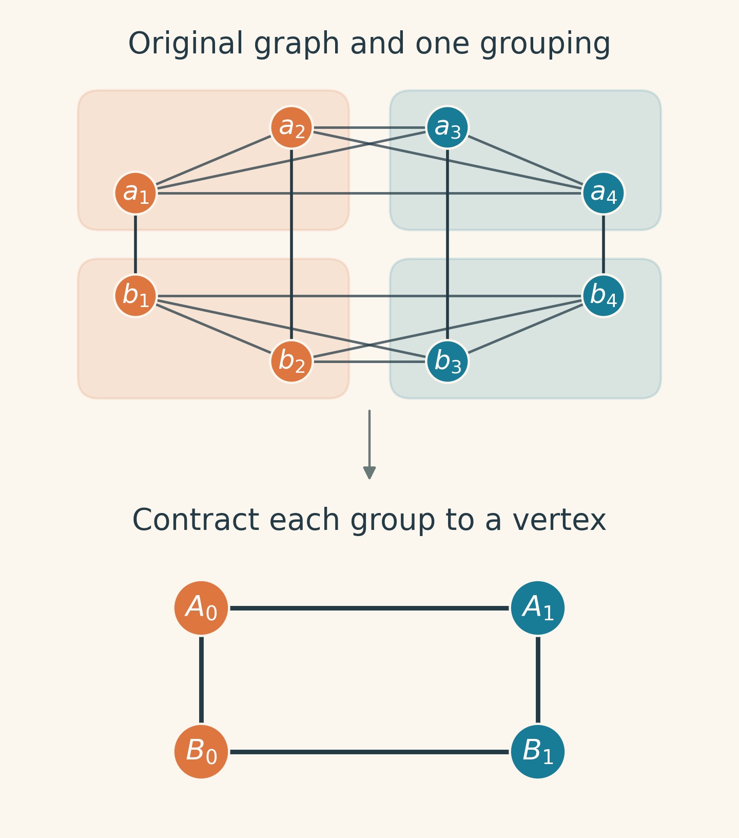
The construction begins with two vertices for each bead, one in the upper row and one in the lower, denoted $a_i$ and $b_i$ , respectively. The subscript $i$ identifies the bead represented by both vertices. All vertices in the upper row are pairwise adjacent, as are all vertices in the lower row; between rows, only corresponding $a_i$ and $b_i$ are joined. Figure 1 shows this base graph for four beads.

Why use two cliques? If a clique is split among three different groups, those three groups will be pairwise adjacent, forming a triangle in the skeleton. Requiring no triangles therefore limits each row to at most two groups.

The matching edges between the rows restrict the choices further. The Gewu researcher proves that only two kinds of valid grouping remain: either each entire row occupies one group, or each row is split into two groups, with corresponding indices in the two rows choosing the same side. A group also cannot mix vertices from the upper and lower rows.

The reason the choices must stay synchronized is easy to see. If two indices in one upper-row group correspond to vertices in two different lower-row groups, those three groups will be pairwise adjacent, forming a triangle. The remaining matching edges and the edges within each row rule out mixing vertices from the two rows. Thus, once the “leave each row intact” case can be excluded, the two rows together can store a consistent choice of two colors.

Consistency alone is not enough, though. Every triple on the list must contain both colors. The paper uses a very short path to check this.

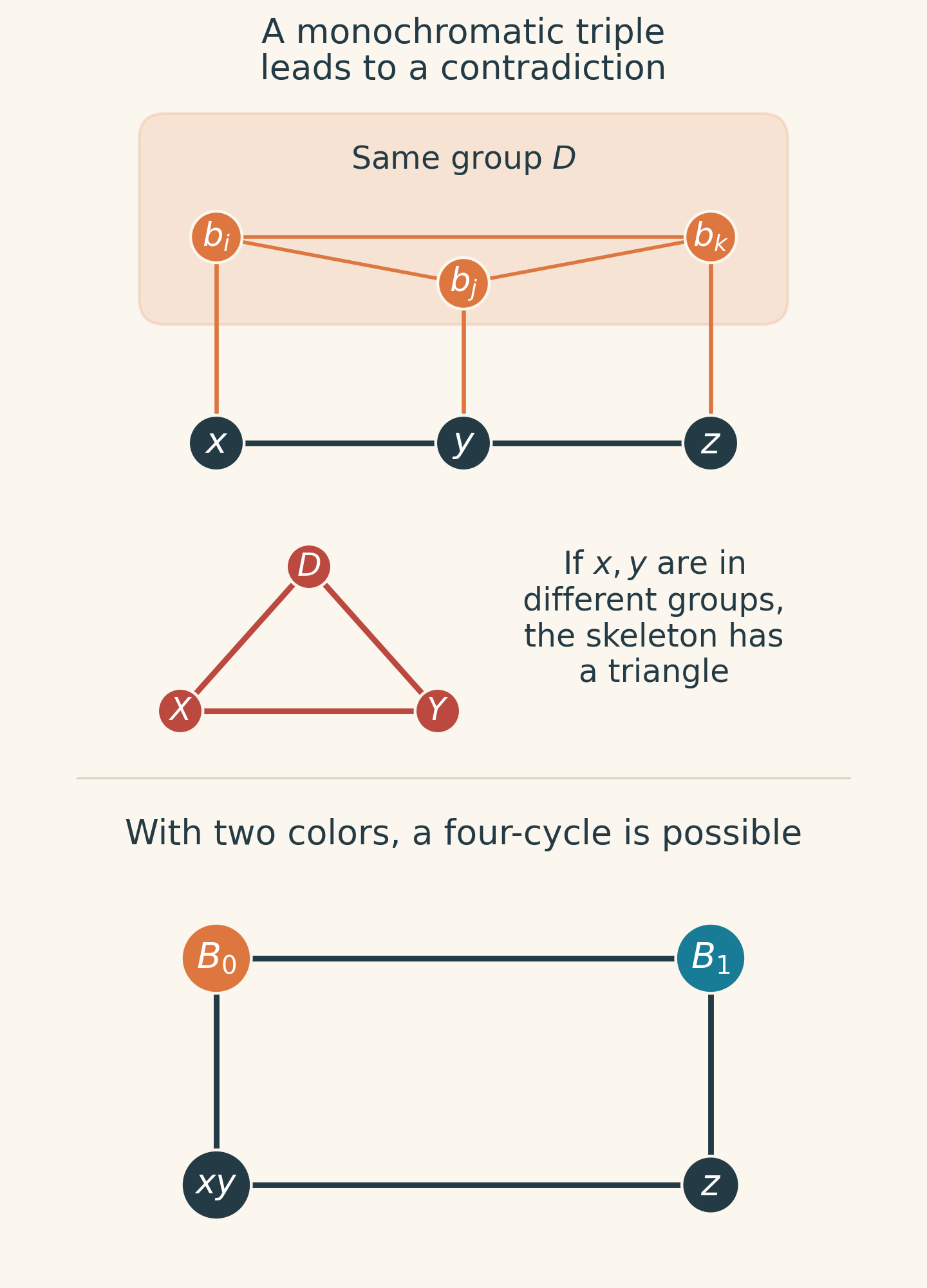
For three beads with specified indices $i,j,k$ , add three vertices $x,y,z$ , join them only into the path $x$ — $y$ — $z$ , and connect them to the lower-row vertices $b_i,b_j,b_k$ , respectively. Add no edges between paths belonging to different triples. In particular, remember that there is no edge between the endpoints $x$ and $z$ .

Suppose this triple is monochromatic. The three corresponding lower-row vertices then belong to a single group, denoted $D$ . None of the three path vertices can enter $D$ : each is adjacent to only one of those lower-row vertices, so it cannot meet the requirement that every pair within a group be adjacent. Yet the groups containing the path vertices are all connected to $D$ .

Now consider the adjacent vertices $x$ and $y$ . If they belong to different groups, there is an edge between those groups, and both are connected to $D$ , producing a triangle in the skeleton. To avoid a triangle, $x$ and $y$ must therefore be placed in the same group. The same reasoning forces $y$ and $z$ into the same group as well.

All three path vertices are thus forced together, but their two endpoints are not adjacent, so they cannot form a clique. This is a contradiction: a monochromatic triple cannot correspond to a valid model. If the entire lower row is left intact, any triple produces the same contradiction, so that grouping is excluded too.

At the top, three lower-row vertices in the same group are each joined to a vertex of a three-vertex path; placing adjacent path vertices in different groups creates a triangle. Below, a grouping with two colors yields a four-cycle after the first two path vertices are merged — Figure 3: In the upper half, the three lower-row vertices are assumed to belong to the same group $D$ . In the small triangle, $X,Y$ denote the groups containing $x,y$ , respectively: whenever these groups differ, the triangle appears. The lower half shows one valid case with two colors: the first two indices belong to $B_0$ , and the third to $B_1$ . Contracting the adjacent $x,y$ into a single vertex and leaving $z$ in a group of its own produces exactly a four-cycle, together with the existing $B_0$ — $B_1$ edge. The diagram shows only the local relationships involving one triple. Drawn from Section 5 of the paper.

At this point, we know that if a skeleton meeting the requirements exists, we can read a valid coloring from its grouping. But a reduction needs the other direction too. If the beads can indeed be colored correctly, the constructed graph must actually admit such a simple skeleton.

In a triple containing both colors, two indices always share a color. If they correspond to adjacent vertices on the path, merge those two path vertices into one group and leave the remaining vertex in a group of its own. The local skeleton is a four-cycle, as in Figure 3. If instead the matching colors correspond to the two endpoints, put each of the three path vertices in its own group. The resulting five-vertex graph can be split into two sides, with two vertices on one side and three on the other. Every vertex on one side is adjacent to every vertex on the other, and there are no edges within either side: this is the graph known as $K_{2,3}$ .

The key is that, however many triples there are, these small graphs attach to the rest only through the two lower-row groups, which already have an edge between them. Each small graph contains no triangles, and there are no edges between paths from different triples, so joining them introduces no triangles either. The Gewu researcher also gives an explicit tree decomposition for the entire skeleton: start with the base four-cycle and attach the bags of each local graph, with no bag containing more than three vertices. Thus, when all the local conditions are met at once, the overall treewidth remains at most two. The small size of the local structures really does carry over to the whole.

This locks the two problems together: the list of triples has a valid two-coloring if and only if the constructed graph has a grouping and skeleton meeting the requirements. Each bead needs only two base vertices, each triple adds only three path vertices, and the number of edges within the rows grows only quadratically with the number of beads. The size of the reduction is bounded by a polynomial. If we could recognize the skeletons efficiently in general, we could solve the original coloring problem just as efficiently.

On the other hand, a candidate grouping, a skeleton, and a tree decomposition with at most three vertices per bag can be checked item by item: are the vertices in each group pairwise adjacent, are all edges between groups recorded, are there any triangles, and do the bags meet the coverage and connectivity requirements? Verification also takes only polynomial time. The hardness reduction and the easily verified certificate together establish NP-completeness.

The work thus draws a clear boundary. When the skeleton is required to have no triangles, recognition is solvable in polynomial time for a treewidth bound of zero or one; for any fixed treewidth bound of at least two, recognition is NP-complete. The latter claim does not follow simply from the idea that “relaxing the conditions cannot make the problem easier.” The skeleton obtained from a valid coloring in the proof already has treewidth two, while the argument that recovers a coloring from any candidate model uses only the absence of triangles. The same reduction therefore works across these larger bounds.

This boundary concerns general algorithms with no restriction on the input graph. It still leaves specific questions for further research: which restricted classes of input graphs allow efficient recognition? If the size of the hidden skeleton is also restricted, how much can that constrain the search? Answering these questions will require new algorithms and proofs; the present hardness result does not settle these cases.

Returning to that densely connected graph of relationships, we can now see how many choices separate “having a simple skeleton” from “being able to find it easily.” A four-cycle is not itself complex, nor is a decomposition with three vertices per bag large. Yet deciding who belongs in a group with whom, so that all triples are satisfied at once, is enough to encode an NP-complete problem. Simple structure can help with computation, but it need not reveal itself readily.

Research source: The supplied paper, Recognition of Graphs with Triangle-Free Treewidth-Two Thin Models is NP-Complete, September 1, 2026. Background comes from the original paper by Dyer and Müller linked in the text. All illustrations were drawn programmatically for this article based on the paper. The cover is a conceptual artistic illustration, and the figures in the body are deterministic structural diagrams; none represents experimental data.